In this post (based on a talk I gave at R in Finance 2018. The videos haven’t been posted yet but I’ll add a link when they have been), we lay the groundwork for a Shiny dashboard that allows a user to construct a portfolio, choose a set of Fama French factors, regress portfolio returns on the Fama French factors and visualize the results.
The final app is viewable here.
Before we get to Shiny, let’s walk through how to do this in a Notebook, to test our functions, code and results before wrapping it into an interactive dashboard. Next time, we will port to Shiny.
We will work with the following assets and weights to construct a portfolio:
+ SPY (S&P500 fund) weighted 25%
+ EFA (a non-US equities fund) weighted 25%
+ IJS (a small-cap value fund) weighted 20%
+ EEM (an emerging-mkts fund) weighted 20%
+ AGG (a bond fund) weighted 10%
Get Daily Returns and Build Portfolio
First, we import daily prices from a relatively new data source, tiingo, making use of the riingo package (a good vignette for which is here). I just started using tiingo and have really liked its performance thus far, plus it seems that fundamental data may be in the offing.
The first step is to create an API key and riingo makes that quite convenient:
riingo_browse_signup()
# This requires that you are signed in on the site once you sign up
riingo_browse_token()
Then we set our key for use this session with:
# Need an API key for tiingo

riingo_set_token("your api key here")
Now we can start importing prices. Let’s first choose our 5 tickers and store them in a vector called symbols.
# The symbols vector holds our tickers.
symbols <- c("SPY","EFA", "IJS", "EEM","AGG")
And now use the riingo_prices() function to get our daily prices. Note that we can specify a start_date and could have chosen an end_date as well.
I want to keep only the tickers, dates and adjusted closing prices and will use dplyr's select() function to keep those columns. This is possible because riingo_prices() returned a tidy tibble.
# Get daily prices.
prices_riingo <-
  riingo_prices(symbols,
                start_date = "2013-01-01") %>%
  select(ticker, date, adjClose)
We convert to log returns using mutate(returns = (log(adjClose) - log(lag(adjClose)))).
# Convert to returns
returns_riingo <-
  prices_riingo %>%
  group_by(ticker) %>%
  mutate(returns = (log(adjClose) - log(lag(adjClose))))
Next we want to convert those individual returns to portfolio returns, and that means choosing portfolio weights.
# Create a vector of weights
w <- c(0.25, 0.25, 0.20, 0.20, 0.10)
And now we pass the individual returns and weights to dplyr.
# Create a portfolio and calculate returns
portfolio_riingo <-
  returns_riingo %>%
  mutate(weights = case_when(
    ticker == symbols[1] ~ w[1],
    ticker == symbols[2] ~ w[2],
    ticker == symbols[3] ~ w[3],
    ticker == symbols[4] ~ w[4],
    ticker == symbols[5] ~ w[5]),
  weighted_returns = returns * weights) %>%
  group_by(date) %>%
  summarise(returns = sum(weighted_returns))

head(portfolio_riingo)
## # A tibble: 6 x 2
## date returns
## <dttm> <dbl>
## 1 2013-01-02 00:00:00 NA
## 2 2013-01-03 00:00:00 - 0.00497
## 3 2013-01-04 00:00:00 0.00441
## 4 2013-01-07 00:00:00 - 0.00452
## 5 2013-01-08 00:00:00 - 0.00460
## 6 2013-01-09 00:00:00 0.00327We could have converted to portfolio returns using tq_portfolio() from the tidyquant package. That probably would be better if we had 100 assets and 100 weights and did not want to grind through those case_when() lines above. Still, I like to run the portfolio once via the more verbose dplyr method because it forces me to walk through the assets and their weights.
Here is the more succinct tq_portfolio() version.
portfolio_returns_tq <-
  returns_riingo %>%
  tq_portfolio(assets_col  = ticker,
               returns_col = returns,
               weights     = w,
               col_rename  = "returns")

head(portfolio_returns_tq)
## # A tibble: 6 x 2
## date returns
## <dttm> <dbl>
## 1 2013-01-02 00:00:00 0
## 2 2013-01-03 00:00:00 -0.00497
## 3 2013-01-04 00:00:00 0.00441
## 4 2013-01-07 00:00:00 -0.00452
## 5 2013-01-08 00:00:00 -0.00459
## 6 2013-01-09 00:00:00 0.00326Importing daily prices and converting to portfolio returns is not a complex job, but it’s still good practice to detail the steps for when our future self or a colleague wishes to revisit this work in 6 months. We will also see how these code flow gets ported almost directly over to our Shiny application.
Importing and Wrangling the Fama French Factors
Next we need to import Fama French factor data, luckily, Ff make their factor data available on their website. We are going to document each step for importing and cleaning this data, to an extent that might be overkill. It can be a grind to document these steps now, but a time saver later when we need to update our Shiny app or Notebook. If someone else needs to update our work in the future, detailed data import steps are crucial.
Have a look at the website where factor data is available.
http://mba.tuck.dartmouth.edu/pages/faculty/ken.french/data_library.html
The data are packaged as zip files so we’ll need to do a bit more than call read_csv().
We will use the tempfile() function from base R to create a variable called temp, and will store the zipped file there.
Now we invoke downloadfile(), pass it the URL address of the zip, which for daily Global 5 Factors is “http://mba.tuck.dartmouth.edu/pages/faculty/ken.french/ftp/Global_5_Factors_Daily_CSV.zip”.
However, I choose not to pass that URL in directly, instead I paste it together in pieces with
factors_input <- "Global_5_Factors_Daily"
factors_address <- paste("http://mba.tuck.dartmouth.edu/pages/faculty/ken.french/ftp/", factors_input, "_CSV.zip", sep="" )
The reason for that is eventually we want to give the user the ability to choose different factors in the Shiny app, meaning the user is choosing a different URL end point depending on which zip is chosen.
We will enable that by having the user choose a different factors_input variable, that then gets pasted to the URL for download. We can toggle over to the Shiny app and see how this looks as a user input.
Next we unzip that data with the unz() function read and the csv file using read_csv().
factors_input <- "Global_5_Factors_Daily"

factors_address <-
  paste("http://mba.tuck.dartmouth.edu/pages/faculty/ken.french/ftp/",
        factors_input,
        "_CSV.zip",
        sep="" )

factors_csv_name <- paste(factors_input, ".csv", sep="")

temp <- tempfile()

download.file(
  # location of file to be downloaded
  factors_address,
  # where we want R to store that file
  temp)

Global_5_Factors <-
  read_csv(unz(temp, factors_csv_name))

head(Global_5_Factors)
## # A tibble: 6 x 1
## `This file was created using the 201804 Bloomberg database.`
## <chr>
## 1 Missing data are indicated by -99.99.
## 2 <NA>
## 3 19900702
## 4 19900703
## 5 19900704
## 6 19900705Have a quick look and notice that the object is not at all what we were expecting.
We need to clean up the metadata by skipping a few rows with skip = 6. Each time we access data from a new source there can be all sorts of maintenance to be performed. And we need to document it!
Global_5_Factors <-
  read_csv(unz(temp, factors_csv_name),
           skip = 6 )

head(Global_5_Factors)
## # A tibble: 6 x 7
## X1 `Mkt-RF` SMB HML RMW CMA RF
## <int> <dbl> <dbl> <dbl> <dbl> <dbl> <dbl>
## 1 19900702 0.700 -0.0600 -0.310 0.220 0.0400 0.0300
## 2 19900703 0.180 0.0800 -0.170 0.0700 0.0400 0.0300
## 3 19900704 0.630 -0.190 -0.160 -0.0700 0.0300 0.0300
## 4 19900705 -0.740 0.310 0.170 -0.130 0.0600 0.0300
## 5 19900706 0.200 -0.150 0.0200 0.200 -0.0300 0.0300
## 6 19900709 0.240 0.180 0.0100 0.0400 -0.240 0.0300Notice the format of the X1 column, which is the date. That doesn’t look like it will play nicely with our date format for portfolio returns. We can change the name of the column with rename(date = X1) and coerce to a nicer format with ymd(parse_date_time(date, "%Y%m%d")) from the lubridate package.
Global_5_Factors <-
  read_csv(unz(temp, factors_csv_name), skip = 6 ) %>%
  rename(date = X1, MKT = `Mkt-RF`) %>%
  mutate(date = ymd(parse_date_time(date, "%Y%m%d")))

head(Global_5_Factors)
## # A tibble: 6 x 7
## date MKT SMB HML RMW CMA RF
## <date> <dbl> <dbl> <dbl> <dbl> <dbl> <dbl>
## 1 1990-07-02 0.700 -0.0600 -0.310 0.220 0.0400 0.0300
## 2 1990-07-03 0.180 0.0800 -0.170 0.0700 0.0400 0.0300
## 3 1990-07-04 0.630 -0.190 -0.160 -0.0700 0.0300 0.0300
## 4 1990-07-05 -0.740 0.310 0.170 -0.130 0.0600 0.0300
## 5 1990-07-06 0.200 -0.150 0.0200 0.200 -0.0300 0.0300
## 6 1990-07-09 0.240 0.180 0.0100 0.0400 -0.240 0.0300It looks good, but there’s one problem. Fama French have their factors on a different scale from our monthly returns - their daily risk free rate is .03. We need to divide the FF factors by 100. Let’s do that with mutate_if(is.numeric, funs(. / 100)).
Global_5_Factors <-
  read_csv(unz(temp, factors_csv_name), skip = 6 ) %>%
  rename(date = X1, MKT = `Mkt-RF`) %>%
  mutate(date = ymd(parse_date_time(date, "%Y%m%d")))%>%
  mutate_if(is.numeric, funs(. / 100))

tail(Global_5_Factors)
## # A tibble: 6 x 7
## date MKT SMB HML RMW CMA RF
## <date> <dbl> <dbl> <dbl> <dbl> <dbl> <dbl>
## 1 2018-04-23 -0.00240 -0.00350 0.00240 0.000300 0.00250 0.000100
## 2 2018-04-24 -0.00530 0.00450 0.00730 -0.00180 0.00370 0.000100
## 3 2018-04-25 -0.00350 -0.00320 -0.000500 0.00150 -0.000400 0.000100
## 4 2018-04-26 0.00650 -0.00400 -0.00620 0.000200 -0.00500 0.000100
## 5 2018-04-27 0.00210 -0.00120 -0.00170 0.00220 -0.000800 0.000100
## 6 2018-04-30 -0.00460 0.00150 0 -0.000500 -0.000800 0.000100Here we display the end of the Fama French observations and can see that they are not updated daily. The data run through the end of April 2018. We will need to deal with that when running our analysis.
In general, our Fama French data object looks good and we were perhaps a bit too painstaking about the path from zipped CSV to readable data frame object.
This particular path can be partly reused for other zipped filed but the more important idea is to document the data provenance that sits behind a Shiny application or any model that might be headed to production. It is a grind in the beginning but a time saver in the future. We can toggle over to the Shiny application and see how this is generalized to whatever Fama French series is chosen by the user.
To the Analysis
We now have two objects, portfolio_riingo and Global_5_Factors, and we want to regress a dependent variable from the former on several independent variables from the latter.
To do that, we can combine them into one object and use mutate() to run the model. It’s a two step process to combine them. Let’s use left_join() to combine them based on the column they have in common, date.
Not only will this create a new object for us, it acts as a check that the dates line up exactly because wherever they do not, we will see an NA.
portfolio_riingo_joined <-
  portfolio_riingo %>%
  mutate(date = ymd(date)) %>%
  left_join(Global_5_Factors) %>%
  mutate(Returns_excess = returns - RF) %>%
  na.omit()

head(portfolio_riingo_joined)
## # A tibble: 6 x 9
## date returns MKT SMB HML RMW CMA RF
## <date> <dbl> <dbl> <dbl> <dbl> <dbl> <dbl> <dbl>
## 1 2013-01-03 -0.00497 -0.00210 0.00120 0.000600 0.000800 1.30e⁻³ 0
## 2 2013-01-04 0.00441 0.00640 0.00110 0.00560 -0.00430 3.60e⁻³ 0
## 3 2013-01-07 -0.00452 -0.00140 0.00580 0 -0.00150 1.00e⁻⁴ 0
## 4 2013-01-08 -0.00460 -0.00270 0.00180 -0.00120 -0.000200 1.20e⁻³ 0
## 5 2013-01-09 0.00327 0.00360 0.000300 0.00250 -0.00280 1.00e⁻³ 0
## 6 2013-01-10 0.00711 0.00830 -0.00180 0.00420 -0.00220 4.00e⁻⁴ 0
## # ... with 1 more variable: Returns_excess <dbl>tail(portfolio_riingo_joined)## # A tibble: 6 x 9
## date returns MKT SMB HML RMW CMA RF
## <date> <dbl> <dbl> <dbl> <dbl> <dbl> <dbl> <dbl>
## 1 2018-04-23 -0.00184 -0.00240 -0.00350 2.40e⁻³ 3.00e⁻⁴ 2.50e⁻³ 1.00e⁻⁴
## 2 2018-04-24 -0.00581 -0.00530 0.00450 7.30e⁻³ -1.80e⁻³ 3.70e⁻³ 1.00e⁻⁴
## 3 2018-04-25 -0.00153 -0.00350 -0.00320 -5.00e⁻⁴ 1.50e⁻³ -4.00e⁻⁴ 1.00e⁻⁴
## 4 2018-04-26 0.00698 0.00650 -0.00400 -6.20e⁻³ 2.00e⁻⁴ -5.00e⁻³ 1.00e⁻⁴
## 5 2018-04-27 0.00154 0.00210 -0.00120 -1.70e⁻³ 2.20e⁻³ -8.00e⁻⁴ 1.00e⁻⁴
## 6 2018-04-30 -0.00601 -0.00460 0.00150 0 -5.00e⁻⁴ -8.00e⁻⁴ 1.00e⁻⁴
## # ... with 1 more variable: Returns_excess <dbl>Notice that the Fama French factors are not current up to today. For any portfolio prices that were after April 30, 2018, the left_join() put an NA. We cleaned those up with na.omit().
We are finally ready for our substance, testing the Fama French factors. Nothing fancy here, we call do(model = lm(Returns_excess ~ MKT + SMB + HML + RMW + CMA, data = .)) and clean up the results with tidy(model).
ff_dplyr_byhand <-
  portfolio_riingo_joined %>%
  do(model = lm(Returns_excess ~ MKT + SMB + HML + RMW + CMA, data = .)) %>%
  tidy(model)

ff_dplyr_byhand
## term estimate std.error statistic p.value
## 1 (Intercept) -6.290033e-05 7.651511e-05 -0.8220642 4.111873e-01
## 2 MKT 1.011678e+00 1.412620e-02 71.6171391 0.000000e+00
## 3 SMB -2.585826e-01 2.549696e-02 -10.1417033 2.468510e-23
## 4 HML -8.797563e-02 3.608638e-02 -2.4379176 1.490198e-02
## 5 RMW -2.067892e-01 4.369295e-02 -4.7327808 2.450441e-06
## 6 CMA 7.234694e-03 5.239065e-02 0.1380913 8.901891e-01We will display this table in the Shiny app and could probably stop here, but let’s also add some rolling visualizations of model results. To do that, we first need to fit our model on a rolling basis and can use the rollify() function from tibbletime to create a rolling model.
First, we choose a rolling window of 100 and then define our rolling function.
window <- 100

rolling_lm <- rollify(.f = function(Returns_excess, MKT, SMB, HML, RMW, CMA) {
                              lm(Returns_excess ~ MKT + SMB + HML + RMW + CMA)
                           },
                      window = window,
                      unlist = FALSE)
Next we apply that function, which we called rolling_lm() to our data frame using mutate().
rolling_ff <-
  portfolio_riingo_joined %>%
  mutate(rolling_lm = rolling_lm(Returns_excess, MKT, SMB, HML, RMW, CMA)) %>%
  slice(-1:-window)

tail(rolling_ff %>% select(date, rolling_lm))
## # A tibble: 6 x 2
## date rolling_lm
## <date> <list>
## 1 2018-04-23 <S3: lm>
## 2 2018-04-24 <S3: lm>
## 3 2018-04-25 <S3: lm>
## 4 2018-04-26 <S3: lm>
## 5 2018-04-27 <S3: lm>
## 6 2018-04-30 <S3: lm>Notice our object has the model results nested in the rolling_lm column. That is substantively fine, but not ideal for creating visualizations on the fly in Shiny.
Let’s extract that the r.squared with map(..., glance()).
rolling_ff_glance <-
  rolling_ff %>%
  mutate(glanced = map(rolling_lm, glance)) %>%
  unnest(glanced) %>%
  select(date, r.squared)

head(rolling_ff_glance)
## # A tibble: 6 x 2
## date r.squared
## <date> <dbl>
## 1 2013-05-29 0.838
## 2 2013-05-30 0.836
## 3 2013-05-31 0.843
## 4 2013-06-03 0.831
## 5 2013-06-04 0.829
## 6 2013-06-05 0.836Next we visualize with highcharter via the hc_add_series() function. I prefer to pass an xts object to highcharter so first we will coerce to xts.
rolling_r_squared_xts <-
  rolling_ff_glance %>%
  tk_xts(date_var = date)


highchart(type = "stock") %>%
  hc_title(text = "Rolling R Squared") %>%
  hc_add_series(rolling_r_squared_xts, color = "cornflowerblue") %>%
  hc_add_theme(hc_theme_flat()) %>%
  hc_navigator(enabled = FALSE) %>%
  hc_scrollbar(enabled = FALSE)
Now we can port that rolling visualization over to the Shiny app.
It might also be nice to chart the rolling beta for each factor. We already have those stored in our rolling model, we just need to extract them. Let’s invoke tidy() from the broom package, and then unnest().
rolling_ff_tidy <-
  rolling_ff %>%
  mutate(tidied = map(rolling_lm, tidy)) %>%
  unnest(tidied) %>%
  select(date, term, estimate, std.error, statistic, p.value)

head(rolling_ff_tidy)
## # A tibble: 6 x 6
## date term estimate std.error statistic p.value
## <date> <chr> <dbl> <dbl> <dbl> <dbl>
## 1 2013-05-29 (Intercept) -0.000212 0.000294 - 0.721 4.73e⁻ ¹
## 2 2013-05-29 MKT 0.933 0.0662 14.1 6.67e⁻²⁵
## 3 2013-05-29 SMB -0.302 0.0961 - 3.15 2.22e⁻ ³
## 4 2013-05-29 HML -0.264 0.183 - 1.44 1.52e⁻ ¹
## 5 2013-05-29 RMW -0.383 0.228 - 1.68 9.59e⁻ ²
## 6 2013-05-29 CMA -0.380 0.180 - 2.11 3.71e⁻ ²We now have the rolling beta estimates for each factor in the estimate column. Let’s chart with ggplot(). We want each term to get its own color so we group_by(term), then call ggplot() and geom_line().
rolling_ff_tidy %>%
  group_by(term) %>%
  filter(term != "(Intercept)") %>%
  ggplot(aes(x = date, y = estimate, color = term)) +
  geom_line()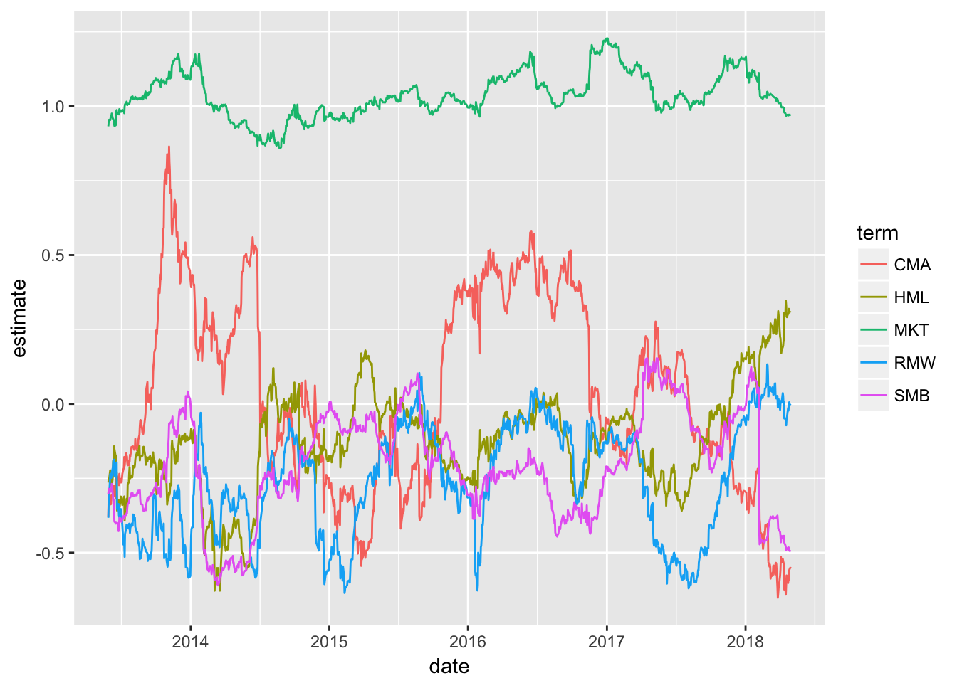
We have grinded through a lot in this Notebook - data import, wrangling, tidying, regression, rolling regression, and visualization - and in so doing have constructed the pieces that will eventually make up our Shiny dashboard.
Next time, we will walk through exactly how to wrap this work into an interactive app. See you then!