Standard Deviation in the xts world

portfolio_sd_xts_builtin <- 
  StdDev(asset_returns_xts, weights = w)


portfolio_sd_xts_builtin_percent <- 
  round(portfolio_sd_xts_builtin * 100, 2)

portfolio_sd_xts_builtin_percent

##      [,1]
## [1,] 2.66

Standard Devation in the tidyverse

portfolio_sd_tidy_builtin_percent <-
  portfolio_returns_dplyr_byhand %>% 
  summarise(
    sd = sd(returns),
    sd_byhand = 
      sqrt(sum((returns - mean(returns))^2)/(nrow(.)-1))) %>% 
  mutate(dplyr = round(sd, 4) * 100,
         dplyr_byhand = round(sd_byhand, 4) * 100)  

Standard Deviation in the tidyquant world

portfolio_sd_tidyquant_builtin_percent <- 
portfolio_returns_tq_rebalanced_monthly %>% 
  tq_performance(Ra = returns, 
                 Rb = NULL, 
                 performance_fun = table.Stats) %>% 
  select(Stdev) %>% 
  mutate(tq_sd = round(Stdev, 4) * 100)

Visualizing Standard Deviation

portfolio_returns_dplyr_byhand %>%
  ggplot(aes(x = date, y = returns)) + 
  geom_point(color = "cornflowerblue") +
  scale_x_date(breaks = pretty_breaks(n = 6)) +
  ggtitle("Scatterplot of Returns by Date") +
  theme(plot.title = element_text(hjust = 0.5))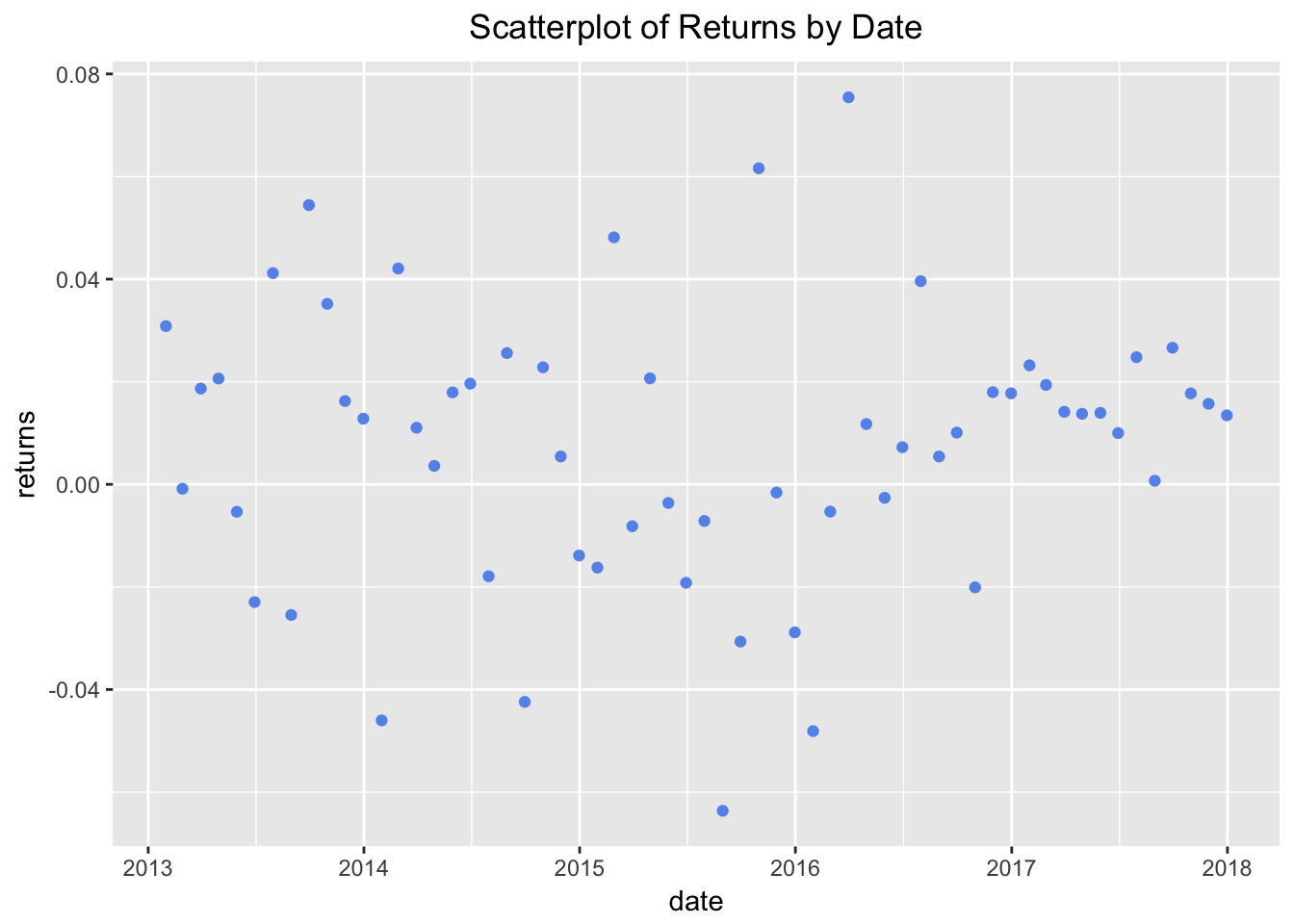

Figure 1: Dispersion of Portfolio Returns

sd_plot <- 
  sd(portfolio_returns_tq_rebalanced_monthly$returns)
mean_plot <- 
  mean(portfolio_returns_tq_rebalanced_monthly$returns)

portfolio_returns_tq_rebalanced_monthly %>%
  mutate(hist_col_red = 
           if_else(returns < (mean_plot - sd_plot), 
                  returns, as.numeric(NA)),
         hist_col_green = 
           if_else(returns > (mean_plot + sd_plot), 
                  returns, as.numeric(NA)),
         hist_col_blue = 
           if_else(returns > (mean_plot - sd_plot) &
                  returns < (mean_plot + sd_plot),
                  returns, as.numeric(NA))) %>% 
  ggplot(aes(x = date)) + 
  
  geom_point(aes(y = hist_col_red),
               color = "red") +
  
  geom_point(aes(y = hist_col_green),
               color = "green") +
  
  geom_point(aes(y = hist_col_blue),
               color = "blue") +
  labs(title = "Colored Scatter", y = "monthly returns") +
  scale_x_date(breaks = pretty_breaks(n = 8)) +
  theme(plot.title = element_text(hjust = 0.5))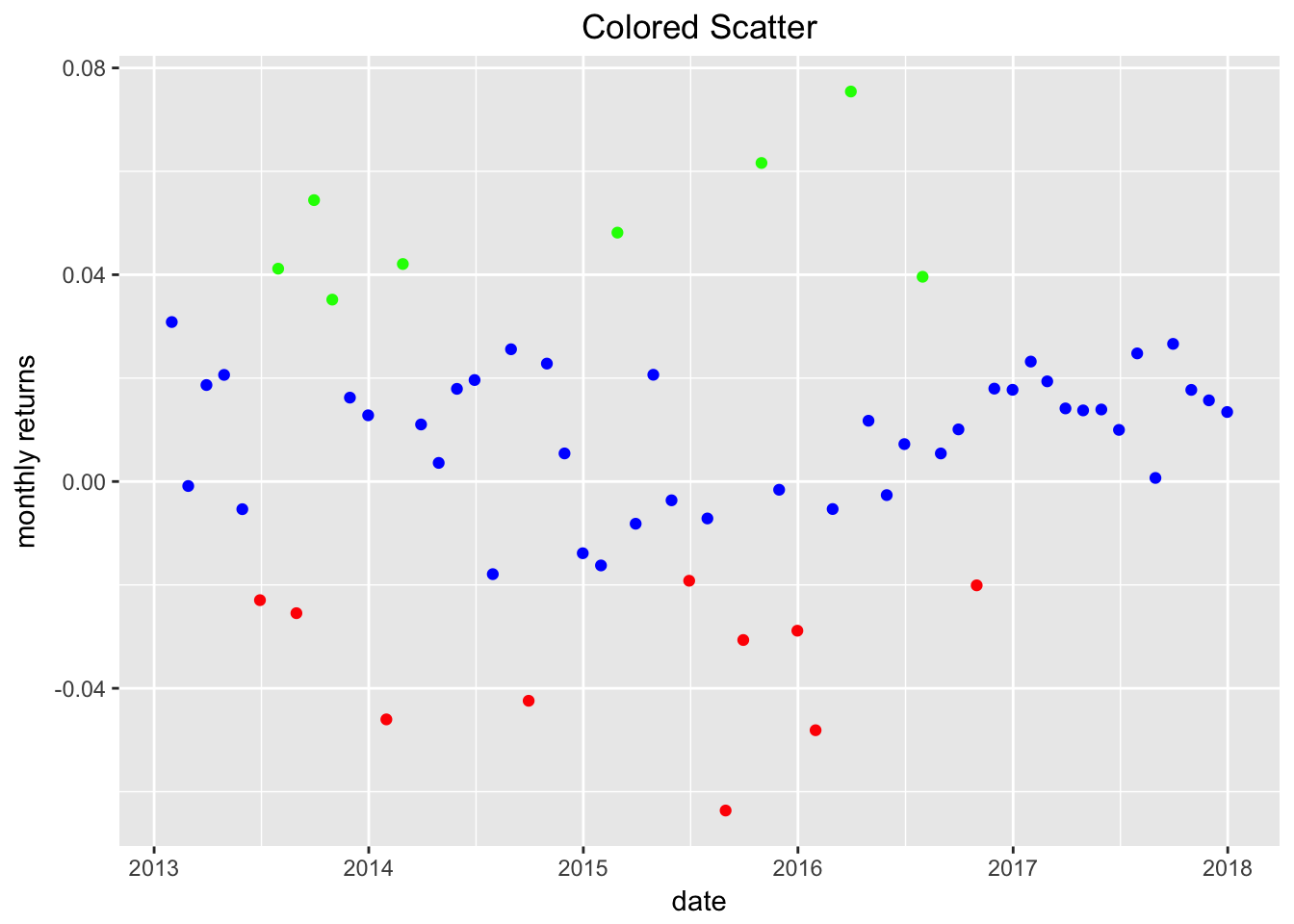

Figure 2: Scatter of Returns Colored by Distance Mean

portfolio_returns_tq_rebalanced_monthly %>%
  mutate(hist_col_red = 
           if_else(returns < (mean_plot - sd_plot), 
                  returns, as.numeric(NA)),
         hist_col_green = 
           if_else(returns > (mean_plot + sd_plot), 
                  returns, as.numeric(NA)),
         hist_col_blue = 
           if_else(returns > (mean_plot - sd_plot) &
                  returns < (mean_plot + sd_plot),
                  returns, as.numeric(NA))) %>% 
  
  ggplot(aes(x = date)) + 
  
  geom_point(aes(y = hist_col_red),
               color = "red") +
  
  geom_point(aes(y = hist_col_green),
               color = "green") +
  
  geom_point(aes(y = hist_col_blue),
               color = "blue") +
  
  geom_hline(yintercept = (mean_plot + sd_plot),
             color = "purple", 
             linetype = "dotted") +
  geom_hline(yintercept = (mean_plot-sd_plot), 
             color = "purple", 
             linetype = "dotted") +
  labs(title = "Colored Scatter with Line", y = "monthly returns") +
  scale_x_date(breaks = pretty_breaks(n = 8)) +
  theme(plot.title = element_text(hjust = 0.5))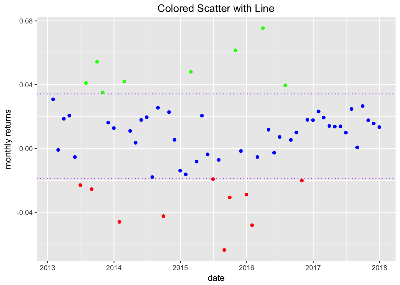

asset_returns_long %>%
  group_by(asset) %>% 
  summarize(sd = 100 * sd(returns)) %>% 
  add_row(asset = "Portfolio", 
          sd = portfolio_sd_tidy_builtin_percent$dplyr) %>% 
  ggplot(aes(x = asset, 
             y = sd, 
             colour = asset)) +
  geom_point() +
 scale_y_continuous(labels = function(x) paste0(x, "%")) +
  geom_text(
        aes(x = "Portfolio", 
            y = 
              portfolio_sd_tidy_builtin_percent$dplyr + .2), 
              label = "Portfolio",
          color = "cornflowerblue")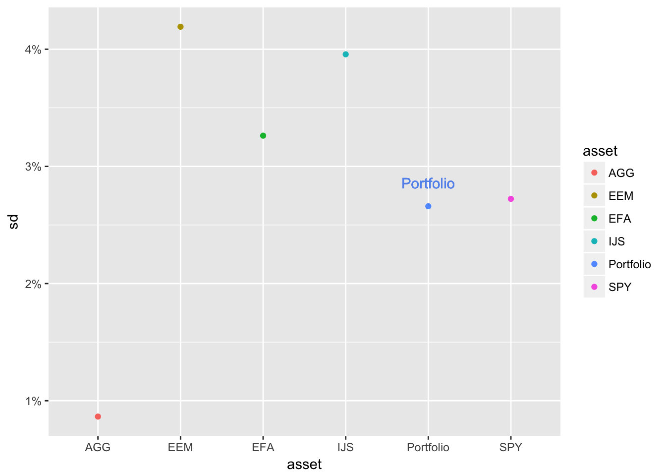

Figure 3: Asset and Portfolio Standard Deviation Comparison

asset_returns_long %>% 
  group_by(asset) %>%
  summarise(expected_return = mean(returns),
            stand_dev = sd(returns)) %>% 
  add_row(asset = "Portfolio",
    stand_dev = 
      sd(portfolio_returns_tq_rebalanced_monthly$returns),
    expected_return = 
      mean(portfolio_returns_tq_rebalanced_monthly$returns)) %>% 
  
  ggplot(aes(x = stand_dev, 
             y = expected_return, 
             color = asset)) +
  geom_point(size = 2) +
  geom_text(
   aes(x = 
    sd(portfolio_returns_tq_rebalanced_monthly$returns) * 1.11, 
      y = 
    mean(portfolio_returns_tq_rebalanced_monthly$returns), 
          label = "Portfolio")) +
  ylab("expected return") +
  xlab("standard deviation") +
  ggtitle("Expected Monthly Returns v. Risk") +
  scale_y_continuous(labels = function(x){ paste0(x, "%")}) +
  # The next line centers the title
  theme_update(plot.title = element_text(hjust = 0.5))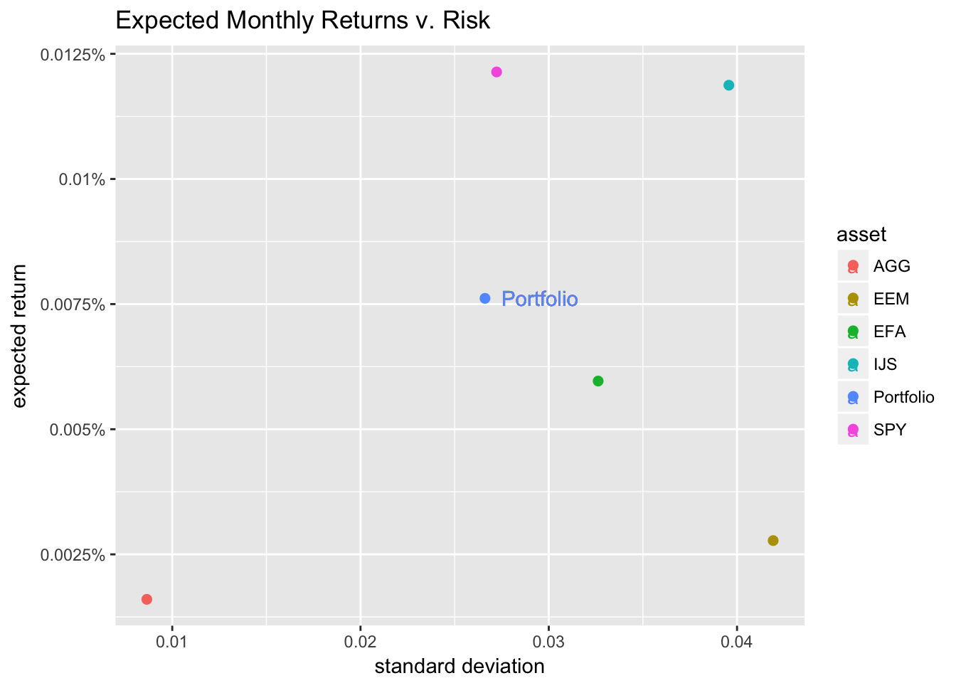

Figure 4: Monthly Returns v. Risk

Rolling Standard Deviation in the xts world

window <- 24

port_rolling_sd_xts <- 
  rollapply(portfolio_returns_xts_rebalanced_monthly,
            FUN = sd,
            width = window) %>% 
  # omit the 23 months for which there is no rolling 24
  # month standard deviation
  na.omit() %>% 
  `colnames<-`("rolling_sd")

tail(port_rolling_sd_xts, 3)

##            rolling_sd
## 2017-10-31 0.02339123
## 2017-11-30 0.02328078
## 2017-12-31 0.02169150

Rolling Standard Devation with the tidyverse and tibbletime

sd_roll_24 <- 
  rollify(sd, window = window)

port_rolling_sd_tidy_tibbletime <- 
  portfolio_returns_tq_rebalanced_monthly %>%
  as_tbl_time(index = date) %>% 
  mutate(sd = sd_roll_24(returns)) %>% 
  select(-returns) %>% 
  na.omit()

tail(port_rolling_sd_tidy_tibbletime, 3)

## # A time tibble: 3 x 2
## # Index: date
##   date           sd
##   <date>      <dbl>
## 1 2017-10-31 0.0234
## 2 2017-11-30 0.0233
## 3 2017-12-31 0.0217

Rolling Standard Deviation in the tidyquant world

port_rolling_sd_tq <- 
  portfolio_returns_tq_rebalanced_monthly %>% 
  tq_mutate(mutate_fun = rollapply,
            width = window,
            FUN = sd,
            col_rename = "rolling_sd") %>%
  select(date, rolling_sd) %>% 
  na.omit()

port_rolling_sd_tidy_tibbletime %>% 
  mutate(sd_tq = port_rolling_sd_tq$rolling_sd,
         sd_xts = round(port_rolling_sd_xts$rolling_sd, 4)) %>% 
  tail(3)

## # A time tibble: 3 x 4
## # Index: date
##   date           sd  sd_tq sd_xts   
##   <date>      <dbl>  <dbl> <S3: xts>
## 1 2017-10-31 0.0234 0.0234 0.0234   
## 2 2017-11-30 0.0233 0.0233 0.0233   
## 3 2017-12-31 0.0217 0.0217 0.0217

Visualizing Rolling Standard Deviation in the xts world

port_rolling_sd_xts_hc <- 
  round(port_rolling_sd_xts, 4) * 100

highchart(type = "stock") %>% 
  hc_title(text = "24-Month Rolling Volatility") %>%
  hc_add_series(port_rolling_sd_xts_hc, 
                color = "cornflowerblue") %>% 
  hc_add_theme(hc_theme_flat()) %>%
  hc_yAxis(
    labels = list(format = "{value}%"), 
             opposite = FALSE) %>%
  hc_navigator(enabled = FALSE) %>% 
  hc_scrollbar(enabled = FALSE) %>% 
  hc_exporting(enabled= TRUE) %>% 
  hc_legend(enabled = TRUE)

Visualizing Rolling Standard Deviation in the tidyverse

port_rolling_sd_tq %>%
  ggplot(aes(x = date)) + 
  geom_line(aes(y = rolling_sd), color = "cornflowerblue") + 
  scale_y_continuous(labels = scales::percent) +
  scale_x_date(breaks = pretty_breaks(n = 8)) +
  labs(title = "Rolling Standard Deviation", y = "") +
    theme(plot.title = element_text(hjust = 0.5))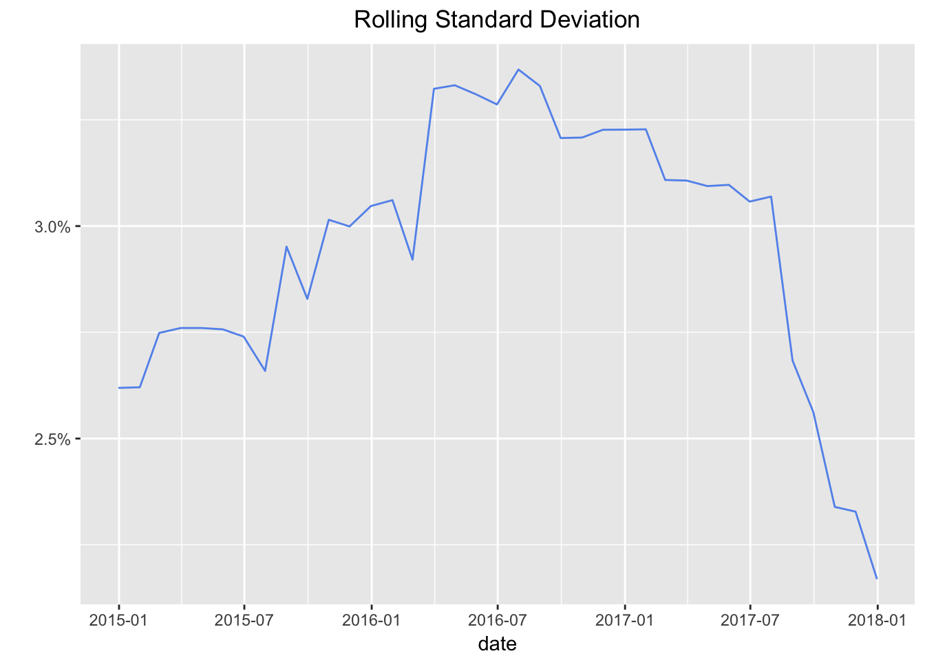

Figure 5: Rolling Volatility ggplot