Load up our packages
install.packages("tidyverse")
install.packages("tidyquant")
install.packages("timetk")
install.packages("tibbletime")
install.packages("broom")
install.packages("dygraphs")

devtools::install_github("jbkunst/highcharter")
library(tidyverse)
library(tidyquant)
library(timetk)
library(tibbletime)
library(scales)
library(highcharter)
library(broom)
library(PerformanceAnalytics)
library(dygraphs)Introducing R
+ Statistical programming language -> by data scientists, for data scientists
+ Base R + 17,000 packages
+ RStudio
+ Shiny
+ sparklyr
+ tensorflow
+ Rmarkdown
+ database connectors
+ htmlwidgets
Packages for finance
library(PerformanceAnalytics)
library(PortfolioAnalytics)
library(TTR)
library(tidyquant)
library(quantmod)
library(xts)
List of packages for finance here: https://cran.r-project.org/web/views/Finance.html
Packages for data visualization
library(ggplot2)
library(dygraphs)
library(highcharter)
library(shiny)
An example project
- Import data for 5 ETFs
- Visualize prices and returns
- Calculate some stats of interest
- Create an SMA 50 v. SMA 200
Run a rolling linear model, chart some results
- SPY (S&P500 fund)
- EFA (a non-US equities fund)
- IJS (a small-cap value fund)
- EEM (an emerging-mkts fund)
- AGG (a bond fund)
Import the Data
+ from excel using `read_excel`

+ from csv using `read_csv`

+ from Yahoo! Finance using `getSymbols` or `tq_get`

+ from myssql, postgres etc using `dbConnect`

+ via API with `httr` and `jsonlite` (important for Alternative Data)
Get data
# The symbols vector holds our tickers.
symbols <- c("SPY",
             "EFA",
             "IJS",
             "EEM",
             "AGG")

# data imported from Yahoo! Finance
etf_prices<-
  tq_get(symbols, from  = "2012-12-31") %>%
  select(symbol, date, adjusted) %>%
  spread(symbol, adjusted) %>%
  tk_xts(date_var = date)
Inspect the data
head(etf_prices) AGG EEM EFA IJS SPY
2012-12-31 97.30676 39.63340 48.20629 74.55437 127.1599
2013-01-02 97.19288 40.41088 48.95237 76.60001 130.4191
2013-01-03 96.94758 40.12492 48.47759 76.49866 130.1244
2013-01-04 97.05273 40.20534 48.72346 77.09759 130.6959
2013-01-07 97.00017 39.90150 48.51151 76.64607 130.3387
2013-01-08 97.08776 39.54404 48.24020 76.35121 129.9637Visualize
dygraph(etf_prices)Another Visualization
highchart(type = "stock") %>%
  hc_add_series(etf_prices[,1]) %>%
  hc_add_series(etf_prices[,2]) %>%
  hc_add_series(etf_prices[,3]) %>%
  hc_add_series(etf_prices[,4]) %>%
  hc_add_series(etf_prices[,5]) %>%
  hc_title(text = "Highcharting 5 ETFS") %>%
  hc_yAxis(opposite = FALSE,
           labels = list(format = "${value}")) %>%
  hc_legend(enabled = TRUE) %>%
  hc_navigator(enabled = FALSE) %>%
  hc_exporting(enabled = TRUE)
Performance Analytics: getting started
etf_returns <-
  Return.calculate(etf_prices, method = "log")

head(etf_returns)
AGG EEM EFA IJS
2012-12-31 NA NA NA NA
2013-01-02 -0.0011710460 0.019426883 0.015358255 0.027068430
2013-01-03 -0.0025270480 -0.007101493 -0.009746094 -0.001323970
2013-01-04 0.0010840087 0.002002185 0.005058969 0.007798811
2013-01-07 -0.0005416977 -0.007585831 -0.004359509 -0.005873638
2013-01-08 0.0009026116 -0.008998854 -0.005608370 -0.003854452
SPY
2012-12-31 NA
2013-01-02 0.025307299
2013-01-03 -0.002261673
2013-01-04 0.004382005
2013-01-07 -0.002736513
2013-01-08 -0.002881389table.Stats(etf_returns) AGG EEM EFA IJS SPY
Observations 1448.0000 1448.0000 1448.0000 1448.0000 1448.0000
NAs 1.0000 1.0000 1.0000 1.0000 1.0000
Minimum -0.0110 -0.0626 -0.0898 -0.0386 -0.0427
Quartile 1 -0.0011 -0.0069 -0.0040 -0.0048 -0.0028
Median 0.0001 0.0005 0.0005 0.0008 0.0007
Arithmetic Mean 0.0001 0.0001 0.0002 0.0005 0.0006
Geometric Mean 0.0001 0.0000 0.0002 0.0005 0.0005
Quartile 3 0.0013 0.0074 0.0053 0.0065 0.0048
Maximum 0.0084 0.0479 0.0327 0.0339 0.0390
SE Mean 0.0001 0.0003 0.0002 0.0002 0.0002
LCL Mean (0.95) 0.0000 -0.0005 -0.0002 0.0001 0.0002
UCL Mean (0.95) 0.0002 0.0007 0.0007 0.0010 0.0010
Variance 0.0000 0.0001 0.0001 0.0001 0.0001
Stdev 0.0020 0.0117 0.0089 0.0094 0.0077
Skewness -0.3176 -0.2652 -1.0628 -0.2618 -0.5979
Kurtosis 1.6349 1.3469 8.4793 0.9114 3.5034table.CAPM(etf_returns, etf_returns$SPY) AGG to SPY EEM to SPY EFA to SPY IJS to SPY SPY to SPY
Alpha 0.0001 -0.0006 -0.0003 0.0000 0.0000
Beta -0.0422 1.1464 0.9690 1.0166 1.0000
Beta+ -0.0297 1.1341 0.8953 0.9174 1.0000
Beta- -0.0412 1.0600 0.9930 0.9401 1.0000
R-squared 0.0266 0.5649 0.6962 0.6872 1.0000
Annualized Alpha 0.0199 -0.1408 -0.0769 -0.0091 0.0000
Correlation -0.1630 0.7516 0.8344 0.8290 1.0000
Correlation p-value 0.0000 0.0000 0.0000 0.0000 0.0000
Tracking Error 0.1307 0.1238 0.0781 0.0836 0.0000
Active Premium -0.1336 -0.1503 -0.0956 -0.0119 0.0000
Information Ratio -1.0226 -1.2134 -1.2251 -0.1422 NaN
Treynor Ratio -0.3139 -0.0029 0.0529 0.1328 0.1469Scatter returns
etf_returns %>%
  tk_tbl(rename_index = "date") %>%
  select(-date) %>%
  gather(symbol, return, -SPY) %>%
  ggplot(aes(x = SPY, y = return, color = symbol)) +
  geom_point(alpha = .5) +
  facet_wrap(~symbol)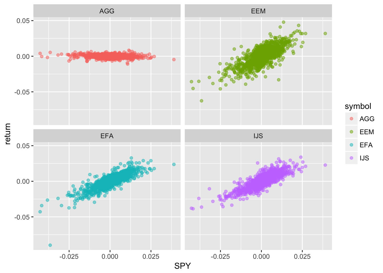
Add regression line
etf_returns %>%
  tk_tbl(rename_index = "date") %>%
  dplyr::select(-date) %>%
  gather(symbol, return, -SPY) %>%
  ggplot(aes(x = SPY, y = return, color = symbol)) +
  geom_point(alpha = .5) +
  geom_smooth(formula = y ~ x, se = TRUE) +
  facet_wrap(~symbol)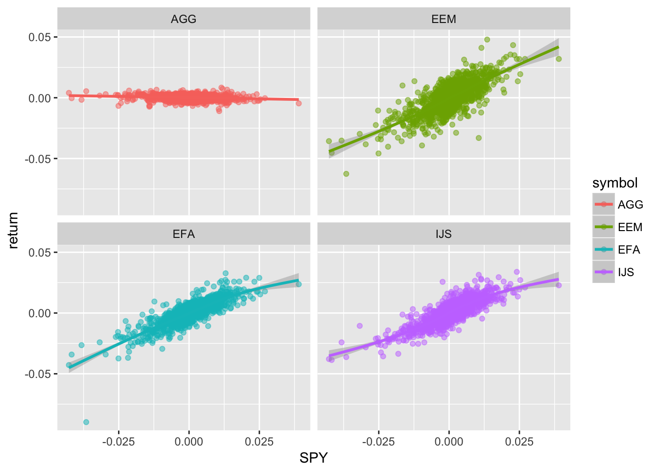
Interactive Scatter
etf_returns %>%
  tk_tbl(rename_index = "date") %>%
  hchart(., type = "scatter", hcaes(x = SPY, y = EEM, date = date)) %>%
  hc_xAxis(title = list(text = "Market Returns"),
           labels = list(format = "{value}%")) %>%
  hc_yAxis(title = list(text = "EEM Returns"),
           labels = list(format = "{value}%")) %>%
  hc_title(text = "Emerging Market v. SPY") %>%
  hc_tooltip(pointFormat = "date: {point.date} <br>
             EEM return: {point.y:.4f}  <br>
             mkt return: {point.x:.4f}")
Grab beta or slope of regression line.
slope <- table.CAPM(etf_returns, etf_returns$SPY)[2, 2]Add the regression line to the original scatter
etf_returns_tibble <-
  etf_returns %>%
  tk_tbl(rename_index = "date")

  hchart(etf_returns_tibble, type = "scatter",
         hcaes(x = SPY, y = EEM, date = date)) %>%
  hc_add_series(etf_returns_tibble, "line",
                hcaes(x = SPY,
                      y = SPY * slope)) %>%
  hc_xAxis(title = list(text = "Market Returns"),
           labels = list(format = "{value}%")) %>%
  hc_yAxis(title = list(text = "EEM Returns"),
           labels = list(format = "{value}%")) %>%
  hc_title(text = "Scatter with Beta Line")
Other Nice Functions (too many to list)
table.DownsideRisk(etf_returns, Rf= .0003) AGG EEM EFA IJS SPY
Semi Deviation 0.0015 0.0085 0.0067 0.0069 0.0057
Gain Deviation 0.0012 0.0070 0.0053 0.0057 0.0049
Loss Deviation 0.0014 0.0080 0.0071 0.0064 0.0061
Downside Deviation (MAR=210%) 0.0085 0.0137 0.0118 0.0118 0.0107
Downside Deviation (Rf=7.56%) 0.0016 0.0087 0.0068 0.0067 0.0056
Downside Deviation (0%) 0.0014 0.0085 0.0066 0.0066 0.0055
Maximum Drawdown 0.0518 0.3794 0.2476 0.2148 0.1399
Historical VaR (95%) -0.0033 -0.0193 -0.0149 -0.0151 -0.0128
Historical ES (95%) -0.0045 -0.0268 -0.0219 -0.0209 -0.0190
Modified VaR (95%) -0.0033 -0.0197 -0.0154 -0.0154 -0.0128
Modified ES (95%) -0.0049 -0.0284 -0.0360 -0.0216 -0.0225table.Drawdowns(etf_returns$EEM) From Trough To Depth Length To Trough Recovery
1 2014-09-08 2016-01-20 2017-09-18 -0.3794 764 345 419
2 2018-01-29 2018-09-10 <NA> -0.2158 172 156 NA
3 2013-01-03 2013-06-24 2014-07-24 -0.1948 392 119 273
4 2017-11-24 2017-12-06 2018-01-02 -0.0533 26 9 17
5 2014-07-29 2014-08-07 2014-08-19 -0.0396 16 8 8SharpeRatio(etf_returns, Rf = .0003) AGG EEM EFA
StdDev Sharpe (Rf=0%, p=95%): -0.12391054 -0.020919066 -0.006924686
VaR Sharpe (Rf=0%, p=95%): -0.07409206 -0.012404382 -0.004008990
ES Sharpe (Rf=0%, p=95%): -0.04986439 -0.008618933 -0.001713013
IJS SPY
StdDev Sharpe (Rf=0%, p=95%): 0.02623972 0.03563936
VaR Sharpe (Rf=0%, p=95%): 0.01599121 0.02144298
ES Sharpe (Rf=0%, p=95%): 0.01141275 0.01215960InformationRatio(etf_returns, etf_returns$SPY) AGG EEM EFA IJS SPY
Information Ratio: SPY -1.022615 -1.213369 -1.225114 -0.1422194 NaNSemiDeviation(etf_returns) AGG EEM EFA IJS SPY
Semi-Deviation 0.001450925 0.008533412 0.006743213 0.006862133 0.005725545Standard Deviation of each asset
StdDev(na.omit(etf_returns)) AGG EEM EFA IJS SPY
StdDev 0.001984284 0.01170326 0.008911274 0.009409863 0.007673235Portfolio Standard Deviation
StdDev(na.omit(etf_returns),
       weights = c(.1, .2, .2, .2, .3))
[,1]
[1,] 0.007505251Contribution to Portfolio Standard Deviation
StdDev(na.omit(etf_returns),
       weights = c(.1, .2, .2, .2, .3),
       portfolio_method = "component")
$StdDev
[1] 0.007505251
$contribution
AGG EEM EFA IJS SPY
-1.886601e-05 2.090247e-03 1.637633e-03 1.625859e-03 2.170378e-03
$pct_contrib_StdDev
AGG EEM EFA IJS SPY
-0.002513708 0.278504648 0.218198318 0.216629513 0.289181229 Visualize Contribution
StdDev(na.omit(etf_returns),
       weights = c(.1, .2, .2, .2, .3),
       portfolio_method = "component") %>%
  as.tibble() %>%
  add_column(symbols = sort(symbols)) %>%
  ggplot(aes(x = symbols, y = pct_contrib_StdDev, fill = symbols)) +
  geom_col(width = .5) +
  labs(y = "percent contribution to vol", x = "", title = "Asset Contribution to Vol") +
  scale_y_continuous(labels = scales::percent)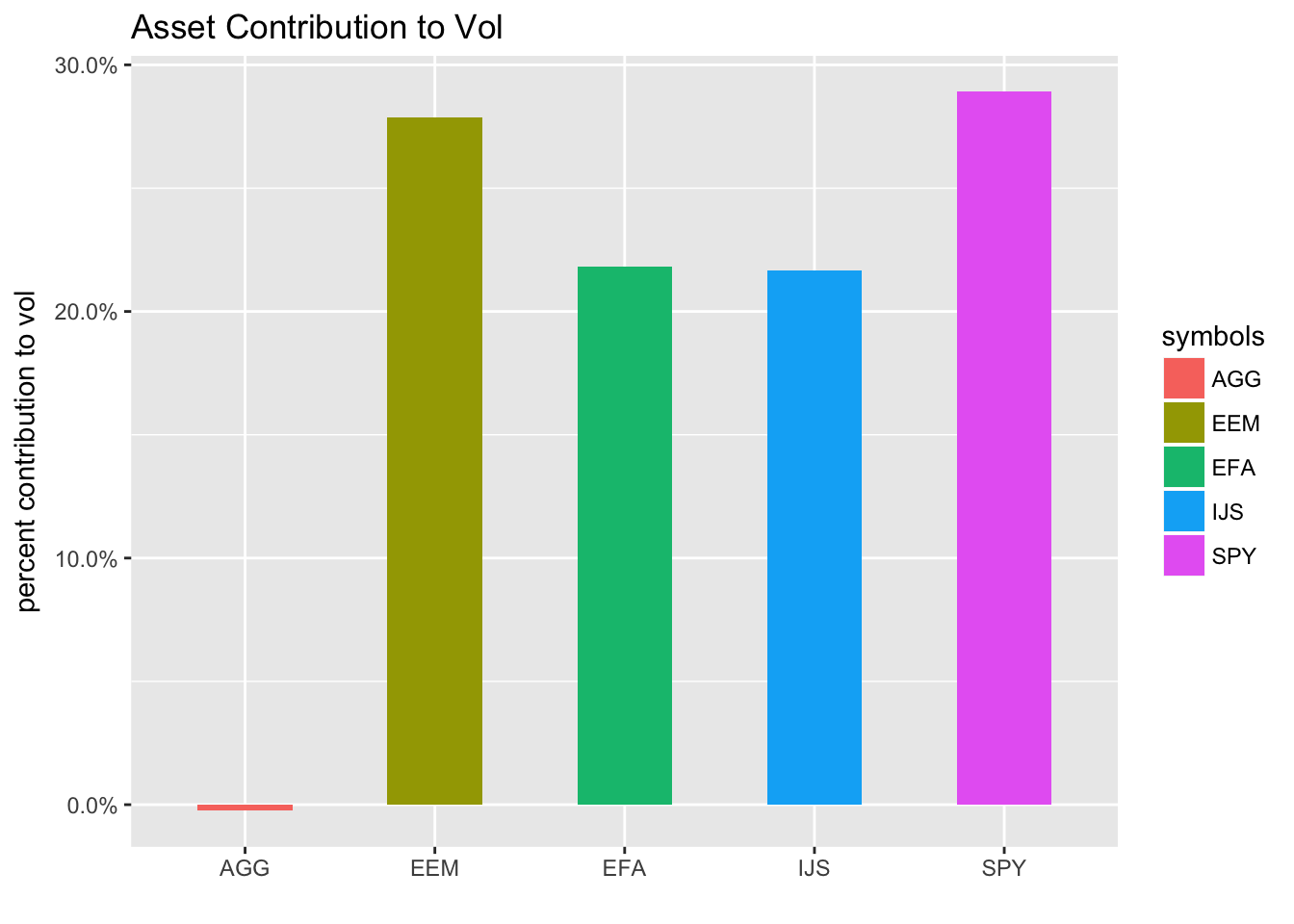
Rolling Mean Calculations and Visualization: our own functions
sma_50 <- rollify(mean, window = 50)
sma_200 <- rollify(mean, window = 200)
sd_50 <- rollify(sd, window = 50)
sd_200 <- rollify(sd, window = 200)

etf_rolling_calculations <-
  etf_prices %>%
  tk_tbl(rename_index = "date") %>%
  select(date, SPY) %>%
  mutate(sma50 = sma_50(SPY),
         sma200 = sma_200(SPY),
         sd200_lower = sma200 - sd_200(SPY),
         sd200_upper = sma200 + sd_200(SPY),
         signal = ifelse(sma50 > sma200, 1, 0)
         ) %>%
  select(-SPY) %>%
  na.omit()
highchart()%>%
hc_add_series(etf_rolling_calculations, type = "line",
hcaes(x = date, y = sma200),
name = "sma200"
) %>%
hc_add_series(etf_rolling_calculations, type = "line",
hcaes(x = date, y = sma50),
name = "sma50",
color = "green") %>%
hc_add_series(etf_rolling_calculations,
type = "arearange",
hcaes(x = date,
low = sd200_lower,
high = sd200_upper),
color = "pink",
alpha = .25,
fillOpacity = 0.3,
showInLegend = FALSE
) %>%
hc_title(text = "SMA 50 v. SMA 200") %>%
hc_xAxis(type = 'datetime') %>%
hc_navigator(enabled = FALSE) %>%
hc_scrollbar(enabled = FALSE) %>%
hc_legend(enabled = TRUE) %>%
hc_exporting(enabled = TRUE) Calculate growth of dollar
SMA trend strategy versus buy and hold
etf_trend <-
  etf_prices %>%
  tk_tbl(rename_index = "date") %>%
  select(date, SPY) %>%
  mutate(sma50 = sma_50(SPY),
         sma200 = sma_200(SPY),
         returns = log(SPY) - log(lag(SPY)),
         signal = ifelse(sma50 > sma200, 1, 0),
         daily_treas = (1 + (2/100)) ^ (1/252) - 1,
         buy_hold_returns = (.9 * returns) + (.1 * daily_treas),
         trend_returns = if_else(lag(signal) == 1, (signal * returns), daily_treas)
         ) %>%
  na.omit() %>%
  mutate(
         trend_growth = accumulate(1 + trend_returns, `*`),
         buy_hold_growth = accumulate(1 + buy_hold_returns, `*`)) %>%
  select(date, trend_growth, buy_hold_growth) %>%
  tk_xts(date_var = date)
Visualize Strategy versus Buy and Hold
  highchart(type = "stock") %>%
  hc_title(text = "Growth") %>%
  hc_add_series(etf_trend$trend_growth, color = "cornflowerblue",  name = "trend") %>%
  hc_add_series(etf_trend$buy_hold_growth, color = "green", name = "buy_hold") %>%
  hc_add_theme(hc_theme_flat()) %>%
  hc_navigator(enabled = FALSE) %>%
  hc_scrollbar(enabled = FALSE) %>%
  hc_legend(enabled = TRUE)
Rolling Models
rolling_lm <- rollify(.f = function(EEM, SPY) {
                              lm(EEM ~ SPY)
                           },
                      window = 100,
                      unlist = FALSE)

etf_returns_tibble %>%
  select(date, EEM, SPY) %>%
  na.omit() %>%
  mutate(rolling_beta = rolling_lm(EEM, SPY)) %>%
  slice(-1:-99) %>%
  mutate(glanced = map(rolling_beta,
                      glance)) %>%
  unnest(glanced)
# A tibble: 1,349 x 15
date EEM SPY rolling_beta r.squared adj.r.squared
<date> <dbl> <dbl> <list> <dbl> <dbl>
1 2013-05-24 -0.00871 -0.000846 <S3: lm> 0.641 0.638
2 2013-05-28 0.00543 0.00597 <S3: lm> 0.623 0.619
3 2013-05-29 -0.0128 -0.00652 <S3: lm> 0.627 0.623
4 2013-05-30 0 0.00369 <S3: lm> 0.627 0.623
5 2013-05-31 -0.0183 -0.0145 <S3: lm> 0.641 0.637
6 2013-06-03 0.0147 0.00549 <S3: lm> 0.635 0.631
7 2013-06-04 -0.0123 -0.00482 <S3: lm> 0.638 0.634
8 2013-06-05 -0.0181 -0.0141 <S3: lm> 0.648 0.645
9 2013-06-06 0.00835 0.00901 <S3: lm> 0.655 0.651
10 2013-06-07 -0.00515 0.0126 <S3: lm> 0.628 0.624
# ... with 1,339 more rows, and 9 more variables: sigma <dbl>,
# statistic <dbl>, p.value <dbl>, df <int>, logLik <dbl>, AIC <dbl>,
# BIC <dbl>, deviance <dbl>, df.residual <int>rolling_model_results <-
etf_returns_tibble %>%
select(date, EEM, SPY) %>%
na.omit() %>%
mutate(rolling_beta = rolling_lm(EEM, SPY)) %>%
slice(-1:-99) %>%
mutate(glanced = map(rolling_beta,
glance)) %>%
unnest(glanced) %>%
select(date, r.squared, adj.r.squared, p.value)
rolling_model_results %>%
hchart(., hcaes(x = date, y = r.squared), type = "line") %>%
hc_title(text = "Rolling R-Squared")Other Packages of Interest
library(forecast) # Good out of the box forecasting tools. Useful for macro trends.
library(h2o) # machine learning libraries
library(keras) # deep learning tensorflow.rstudio.com
library(lime) # for ML white-boxing
library(ranger) # random forest
library(recipes) # for ML preprocessing
library(rsample) # for resampling
library(caret) # classification and regression
library(tidytext) # parse text and mining
library(tidyposterior) # posthoc after resamplingGet Started
Download R: https://cloud.r-project.org/
Download RStudio: www.rstudio.com/products/rstudio/download/#download
datacamp course: www.datacamp.com/tracks/applied-finance-with-r