First, install our packages:
install.packages("tidyverse")
install.packages("tidyquant")
install.packages("timetk")
install.packages("tibbletime")
install.packages("scales")
install.packages("broom")
devtools::install_github("jbkunst/highcharter")Introducing R and RStudio
+ Statistical programming language -> by data scientists, for data scientists
+ Base R + 17,000 packages
+ RStudio
+ ShinyPackages for today
library(tidyverse)
library(tidyquant)
library(timetk)
library(tibbletime)
library(scales)
library(highcharter)
library(broom)
library(PerformanceAnalytics)List of packages for finance here: https://cran.r-project.org/web/views/Finance.html
Today’s project
+ Buy when the SP500 50-day SMA is above the 200-day SMA (a 'golden cross')
+ Sell when the 50-day SMA moves below the 200-day SMA (a 'death cross').
+ Code up that strategy
+ visualiize its results and descriptive statistics
+ Compare it to buy-and-hold, add secondary logic, visualize that strategy
+ Conclude by building a Shiny dashboard for further explorationImport data
We will be working with SP500 and treasury bills data so that when we exit the SP500 we can invest in treasuries and get some return.
We can use the tidyquant package and it’s tq_get() function to grab the data from yahoo! finance.
symbols <- c("^GSPC", "^IRX")
prices <-
tq_get(symbols,
get = "stock.prices",
from = "1990-01-01")
head(prices)# A tibble: 6 x 8
symbol date open high low close volume adjusted
<chr> <date> <dbl> <dbl> <dbl> <dbl> <dbl> <dbl>
1 ^GSPC 1990-01-02 353. 360. 352. 360. 162070000 360.
2 ^GSPC 1990-01-03 360. 361. 358. 359. 192330000 359.
3 ^GSPC 1990-01-04 359. 359. 353. 356. 177000000 356.
4 ^GSPC 1990-01-05 356. 356. 351. 352. 158530000 352.
5 ^GSPC 1990-01-08 352. 354. 351. 354. 140110000 354.
6 ^GSPC 1990-01-09 354. 354. 350. 350. 155210000 350.Let’s see how to import this data from an Excel file or a csv file if that were desired.
prices_excel <-
read_excel("prices.xlsx") %>%
mutate(date = ymd(date))prices_csv <-
read_csv("prices.csv") %>%
mutate(date = ymd(date))Explore the raw data
Start with the simple line chart.
prices %>%
filter(symbol == "^GSPC") %>%
hchart(.,
hcaes(x = date, y = adjusted),
type = "line") %>%
hc_title(text = "GSPC prices")Now we have our raw data and it looks like there are no issues with it.
Calculate Returns
We will use select(), rename, and mutate() from the dplyr package to calculate returns, then table.Stats() from PerformanceAnayltics to get some quick stats.
prices %>%
select(symbol, date, adjusted) %>%
spread(symbol, adjusted) %>%
rename(sp500 = `^GSPC`, treas = `^IRX`) %>%
mutate(sp500_returns = log(sp500) - log(lag(sp500)),
daily_treas = (1 + (treas/100)) ^ (1/252) - 1) %>%
select(date, sp500_returns, daily_treas) %>%
tq_performance(Ra = sp500_returns,
performance_fun = table.Stats) %>%
t() %>%
knitr::kable()| ArithmeticMean | 0.0003 |
| GeometricMean | 0.0002 |
| Kurtosis | 8.9812 |
| LCLMean(0.95) | 0.0000 |
| Maximum | 0.1096 |
| Median | 0.0005 |
| Minimum | -0.0947 |
| NAs | 1.0000 |
| Observations | 7243.0000 |
| Quartile1 | -0.0044 |
| Quartile3 | 0.0055 |
| SEMean | 0.0001 |
| Skewness | -0.2644 |
| Stdev | 0.0110 |
| UCLMean(0.95) | 0.0005 |
| Variance | 0.0001 |
We calculated returns and demnostrated 4 of the most common data wrangling functions. We also transformed our data, it’s not raw anymore. Let’s visualize our transformation with a scatter plot by calling geom_point().
prices %>%
select(symbol, date, adjusted) %>%
spread(symbol, adjusted) %>%
rename(sp500 = `^GSPC`, treas = `^IRX`) %>%
mutate(sp500_returns = log(sp500) - log(lag(sp500))) %>%
ggplot(aes(x = date, y = sp500_returns)) +
geom_point(color = "cornflowerblue") +
scale_x_date(breaks = pretty_breaks(n = 30)) +
labs(title = "SP500 daily returns",
y = "daily percent") +
theme(axis.text.x = element_text(angle = 90))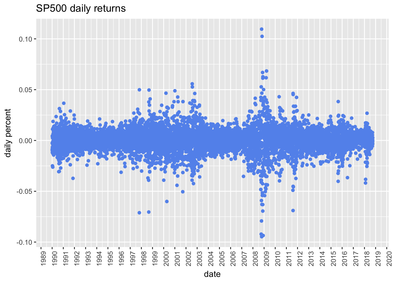
Look at 2000-2002 and late 2008 to 2009.
Moving Averages: our strategy
To start exploring the SMA 50 v SMA 200 strategy, we need to calculate the rolling 50 and 200-day moving averages. Up until now, we have been using built-in functions from various R packages. Now we will create our own with rollify(), to run the mean() function into a moving average calculator.
roll_mean_50 <-
rollify(mean, window = 50)
roll_mean_200 <-
rollify(mean, window = 200)Now we use mutate() to add the moving averages to our original data. mutate() adds columns to our data.
prices %>%
select(symbol, date, adjusted) %>%
spread(symbol, adjusted) %>%
rename(sp500 = `^GSPC`, treas = `^IRX`) %>%
mutate(sma_200 = roll_mean_200(sp500),
sma_50 = roll_mean_50(sp500)) %>%
na.omit() %>%
tail(5)# A tibble: 5 x 5
date sp500 treas sma_200 sma_50
<date> <dbl> <dbl> <dbl> <dbl>
1 2018-09-24 2919. 2.12 2752. 2860.
2 2018-09-25 2916. 2.17 2753. 2862.
3 2018-09-26 2906. 2.16 2754. 2864.
4 2018-09-27 2914 2.14 2756. 2866.
5 2018-09-28 2914. 2.15 2757. 2868.Let’s get systematic
What’s our logic: If the 50-day MA is above the 200-day MA, buy the market, else go to the risk free return, or can put to zero if we prefer. For our purposes, we assume no taxes or trading costs. Buy == get the daily return.
What we need:
1) rolling 50-day SMA
2) rolling 200-day SMA
3) if_else logic to create a buy or sell signal
4) sp500 daily returns/treasury daily returns
5) apply the signal to our returns withsignal = if_else(sma_50 > sma_200, 1, 0)
trend_returns = if_else(lag(signal) == 1, (signal * sp500_returns), daily_treas))
prices %>%
select(symbol, date, adjusted) %>%
spread(symbol, adjusted) %>%
rename(sp500 = `^GSPC`, treas = `^IRX`) %>%
mutate(sp500_returns = log(sp500) - log(lag(sp500)),
daily_treas = (1 + (treas/100)) ^ (1/252) - 1,
sma_200 = roll_mean_200(sp500),
sma_50 = roll_mean_50(sp500)) %>%
na.omit() %>%
mutate(signal = if_else(sma_50 > sma_200, 1, 0),
trend_returns = if_else(lag(signal) == 1, (signal * sp500_returns), daily_treas)) %>%
select(-treas, -sp500)# A tibble: 7,018 x 7
date sp500_returns daily_treas sma_200 sma_50 signal
<date> <dbl> <dbl> <dbl> <dbl> <dbl>
1 1990-10-15 0.0106 0.000274 339. 319. 0
2 1990-10-16 -0.0143 0.000274 339. 318. 0
3 1990-10-17 -0.000535 0.000276 338. 317. 0
4 1990-10-18 0.0231 0.000278 338. 317. 0
5 1990-10-19 0.0218 0.000278 338. 316. 0
6 1990-10-22 0.00727 0.000277 338. 316. 0
7 1990-10-23 -0.00765 0.000276 337. 315. 0
8 1990-10-24 0.000768 0.000277 337. 315. 0
9 1990-10-25 -0.00780 0.000275 337. 314. 0
10 1990-10-26 -0.0178 0.000273 337. 313. 0
# ... with 7,008 more rows, and 1 more variable: trend_returns <dbl>We now have a column for our trend strategy returns. Let’s add a buy and hold strategy where we invest 90% in the SP500 and 10% in treasuries and hold it for the duration.
buy_hold_returns = (.9 * sp500_returns) + (.1 * daily_treas)
prices %>%
select(symbol, date, adjusted) %>%
spread(symbol, adjusted) %>%
rename(sp500 = `^GSPC`, treas = `^IRX`) %>%
mutate(
sp500_returns = log(sp500) - log(lag(sp500)),
daily_treas = (1 + (treas/100)) ^ (1/252) - 1,
sma_200 = roll_mean_200(sp500),
sma_50 = roll_mean_50(sp500)) %>%
na.omit() %>%
mutate(signal = if_else(sma_50 > sma_200, 1, 0),
buy_hold_returns = (.9 * sp500_returns) + (.1 * daily_treas),
trend_returns = if_else(lag(signal) == 1, (signal * sp500_returns), daily_treas)) %>%
select(date, trend_returns, buy_hold_returns)# A tibble: 7,018 x 3
date trend_returns buy_hold_returns
<date> <dbl> <dbl>
1 1990-10-15 NA 0.00958
2 1990-10-16 0.000274 -0.0129
3 1990-10-17 0.000276 -0.000454
4 1990-10-18 0.000278 0.0208
5 1990-10-19 0.000278 0.0197
6 1990-10-22 0.000277 0.00657
7 1990-10-23 0.000276 -0.00686
8 1990-10-24 0.000277 0.000719
9 1990-10-25 0.000275 -0.00700
10 1990-10-26 0.000273 -0.0160
# ... with 7,008 more rowsWe can add columns to see dollar growth for our two asset mixes as well. To calculate dollar growth, we add 1 to the daily returns, and then use accumulate().
sma_trend_results <-
prices %>%
select(symbol, date, adjusted) %>%
spread(symbol, adjusted) %>%
rename(sp500 = `^GSPC`, treas = `^IRX`) %>%
mutate(sma_200 = roll_mean_200(sp500),
sma_50 = roll_mean_50(sp500),
signal = if_else(sma_50 > sma_200, 1, 0),
sp500_returns = log(sp500) - log(lag(sp500)),
daily_treas = (1 + (treas/100)) ^ (1/252) - 1,
buy_hold_returns = (.9 * sp500_returns) + (.1 * daily_treas),
trend_returns = if_else(lag(signal) == 1, (signal * sp500_returns), daily_treas)
) %>%
na.omit() %>%
mutate(trend_growth = accumulate(1 + trend_returns, `*`),
buy_hold_growth = accumulate(1 + buy_hold_returns, `*`))
sma_trend_results %>% tail()# A tibble: 6 x 12
date sp500 treas sma_200 sma_50 signal sp500_returns daily_treas
<date> <dbl> <dbl> <dbl> <dbl> <dbl> <dbl> <dbl>
1 2018-09-21 2930. 2.12 2750. 2857. 1 -0.000369 0.0000834
2 2018-09-24 2919. 2.12 2752. 2860. 1 -0.00352 0.0000834
3 2018-09-25 2916. 2.17 2753. 2862. 1 -0.00131 0.0000851
4 2018-09-26 2906. 2.16 2754. 2864. 1 -0.00329 0.0000848
5 2018-09-27 2914 2.14 2756. 2866. 1 0.00276 0.0000840
6 2018-09-28 2914. 2.15 2757. 2868. 1 -0.00000687 0.0000844
# ... with 4 more variables: buy_hold_returns <dbl>, trend_returns <dbl>,
# trend_growth <dbl>, buy_hold_growth <dbl>Visualize our trend strategy results
How does the dollar growth compare? use select() again to isolate our dollar growth columns. then gather() to a tidy format. What’s tidy? Each variable has its own column. That’s different from wide, which is easier for humans to read.
sma_trend_results %>%
select(date, trend_growth, buy_hold_growth) %>%
gather(strategy, growth, -date) %>%
hchart(., hcaes(x = date, y = growth, group = strategy),
type = "line") %>%
hc_tooltip(pointFormat = "{point.strategy}: ${point.growth: .2f}")Table Stats of our strategies
sma_trend_results %>%
select(date, trend_returns, buy_hold_returns) %>%
gather(strategy, returns, -date) %>%
group_by(strategy) %>%
tq_performance(Ra = returns,
performance_fun = table.Stats) %>%
t() %>%
knitr::kable()| strategy | trend_returns | buy_hold_returns |
| ArithmeticMean | 3e-04 | 3e-04 |
| GeometricMean | 3e-04 | 2e-04 |
| Kurtosis | 8.0652 | 9.1202 |
| LCLMean(0.95) | 2e-04 | 1e-04 |
| Maximum | 0.0499 | 0.0986 |
| Median | 1e-04 | 5e-04 |
| Minimum | -0.0711 | -0.0852 |
| NAs | 0 | 0 |
| Observations | 7017 | 7017 |
| Quartile1 | -0.0020 | -0.0039 |
| Quartile3 | 0.0033 | 0.0050 |
| SEMean | 1e-04 | 1e-04 |
| Skewness | -0.5141 | -0.2665 |
| Stdev | 0.0076 | 0.0100 |
| UCLMean(0.95) | 5e-04 | 5e-04 |
| Variance | 1e-04 | 1e-04 |
Part 2: Adding another layer of logic
Let’s get more complicated and add secondary logic.
We can also add a signal, for example a zscore for when market is a number of standard deviations above or below a rolling average.
How would we implement that?
- Calculate a spread
- turn it into a z-score, number of standard deviations scale
- create a signal (back to
ifelse)
trend_z_results <-
prices %>%
select(symbol, date, adjusted) %>%
spread(symbol, adjusted) %>%
rename(sp500 = `^GSPC`, treas = `^IRX`) %>%
mutate(sma_200 = roll_mean_200(sp500),
sma_50 = roll_mean_50(sp500),
sp500_returns = log(sp500) - log(lag(sp500)),
daily_treas = (1 + (treas/100)) ^ (1/252) - 1) %>%
na.omit() %>%
mutate(trend_signal = if_else(sma_50 > sma_200, 1, 0),
z_spread = (sp500 - sma_200),
z_score = (z_spread - mean(z_spread))/sd(z_spread),
z_signal = if_else(
lag(z_score, 1) < -.05 &
lag(z_score, 2) < -.05 &
lag(z_score, 3) < -.05,
0, 1),
trend_z_returns = if_else(lag(trend_signal) == 1 &
z_signal == 1,
(trend_signal * sp500_returns), daily_treas),
trend_returns = if_else(lag(trend_signal) == 1,
(trend_signal * sp500_returns), daily_treas),
buy_hold_returns = (.9 * sp500_returns) + (.1 * daily_treas)) %>%
select(date, trend_signal, z_signal, buy_hold_returns, trend_returns, trend_z_returns, daily_treas) %>%
na.omit() %>%
mutate(
trend_growth = accumulate(1 + trend_returns, `*`),
trend_z_growth = accumulate(1 + trend_z_returns, `*`),
buy_hold_growth = accumulate(1 + buy_hold_returns, `*`))
trend_z_results %>% tail()# A tibble: 6 x 10
date trend_signal z_signal buy_hold_returns trend_returns
<date> <dbl> <dbl> <dbl> <dbl>
1 2018-09-21 1 1 -0.000323 -0.000369
2 2018-09-24 1 1 -0.00316 -0.00352
3 2018-09-25 1 1 -0.00117 -0.00131
4 2018-09-26 1 1 -0.00296 -0.00329
5 2018-09-27 1 1 0.00249 0.00276
6 2018-09-28 1 1 0.00000226 -0.00000687
# ... with 5 more variables: trend_z_returns <dbl>, daily_treas <dbl>,
# trend_growth <dbl>, trend_z_growth <dbl>, buy_hold_growth <dbl>Visualize our trend + z strategy results
trend_z_results %>%
select(date, trend_growth, trend_z_growth, buy_hold_growth, daily_treas) %>%
gather(strategy, growth, -date, -daily_treas) %>%
hchart(., hcaes(x = date, y = growth, group = strategy), type = "line") %>%
hc_tooltip(pointFormat = "{point.strategy}: ${point.growth: .2f}")Our original trend has grown higher, but the z-score logic seems more less prone to large drawdowns becaus it has the extra layer of downside exit logic.
Table Stats of our new strategies
trend_z_results %>%
select(date, trend_returns, trend_z_growth, buy_hold_returns) %>%
gather(strategy, returns, -date) %>%
group_by(strategy) %>%
tq_performance(Ra = returns,
performance_fun = table.Stats) %>%
t() %>%
knitr::kable()| strategy | trend_returns | trend_z_growth | buy_hold_returns |
| ArithmeticMean | 0.0003 | 2.4200 | 0.0003 |
| GeometricMean | 0.0003 | 2.2935 | 0.0002 |
| Kurtosis | 8.0669 | -0.2279 | 9.1226 |
| LCLMean(0.95) | 0.0002 | 2.3984 | 0.0001 |
| Maximum | 0.0499 | 4.9485 | 0.0986 |
| Median | 0.0001 | 2.4349 | 0.0005 |
| Minimum | -0.0711 | 0.9910 | -0.0852 |
| NAs | 0 | 0 | 0 |
| Observations | 7015 | 7015 | 7015 |
| Quartile1 | -0.0020 | 2.0014 | -0.0039 |
| Quartile3 | 0.0033 | 2.8294 | 0.0050 |
| SEMean | 0.0001 | 0.0110 | 0.0001 |
| Skewness | -0.5140 | 0.3492 | -0.2668 |
| Stdev | 0.0076 | 0.9244 | 0.0100 |
| UCLMean(0.95) | 0.0005 | 2.4416 | 0.0005 |
| Variance | 0.0001 | 0.8546 | 0.0001 |
Wrap to Shiny application
www.reproduciblefinance.com/shiny/ib-webinar/