Welcome to another installment of Reproducible Finance!
Inspired by a great visualization in Hands on Time Series with R by Rami Krispin, today we’ll investigate some market structure data and get to know the Midas data source provided by the SEC.
Let’s start by importing data from the SEC website for the 2nd quarter of 2019.
If you navigate to the SEC website here https://www.sec.gov/opa/data/market-structure/market-structure-data-security-and-exchange.html and right click on the link labeled ‘2019 Q2’, you can copy the link address as https://www.sec.gov/files/opa/data/market-structure/metrics-individual-security-and-exchange/individual_security_exchange_2019_q2.zip. That long string is the path to the zip file holding our market structure data for Q2 of 2019. We will start by downloading that zip file and extracting the CSV of market data. Then we will progress to a programmatic way to download all of the market structure data on that page using a custom-built function.
Have a close look at this string and notice that there are two unique pieces of information
https://www.sec.gov/files/opa/data/market-structure/metrics-individual-security-and-exchange/individual_security_exchange_2019_q2.zip: the year and the quarter. In this case, those are equal to 2019 and q2, respectively.
Let’s first create variables to hold those pieces of data.
year <- "2019"
quarter <- "q2"
Now we need to combine those two variables with the rest of the string. We can use paste0 since there are no spaces in this string.
market_structure_data_address <-
paste0("https://www.sec.gov/files/opa/data/market-structure/metrics-individual-security/individual_security_", year, "_", quarter, ".zip")
And here is the string we just created.
market_structure_data_address[1] "https://www.sec.gov/files/opa/data/market-structure/metrics-individual-security/individual_security_2019_q2.zip"Nothing too mind blowing there but note that this same code paradigm can be used for any data housed on a website: find the link address, identify the pieces that are unique, create variables for them, paste them together with the non-unique portions of the string. The date is very often the unique piece of the string, which makes this process not too painful to repeat elsewhere.
Now that we have a web address for the zip file, we need to download it to R.
Let’s first create a temporary file called temp so that we have a place to deposit the download.
temp <- tempfile()Next we call the download.file() function, supply our pasted string variable market_structure_data_address and point to the temp location.
download.file(
  # location of file to be downloaded
  market_structure_data_address,
  # where we want R to store that file
  temp,
  quiet = TRUE)

# tempdir() will show you where this temp file is being stored
Next we need to create a file name, so we can tell vroom() the name of the file to extract from the zip. We will use the quarter and year variables for this as well.
file_name <- paste0(quarter, "_", year, "_all.csv")We can now import our csv file into R using vroom(unzip(temp, filename)). Let’s also pipe straight to janitor::clean_names() to clean up the column names and use a combination of ymd() and parse_date_time() to coerce the dates into a more usable format.
q2_2019 <-
  vroom(unz(temp, file_name)) %>%
  clean_names() %>%
  mutate(date = ymd(parse_date_time(date, "%Y%m%d")))

q2_2019 %>%
  head()
# A tibble: 6 x 19
date security ticker mcap_rank turn_rank volatility_rank price_rank
<date> <chr> <chr> <dbl> <dbl> <dbl> <dbl>
1 2019-04-01 Stock A 10 5 1 9
2 2019-04-01 Stock AA 9 10 6 7
3 2019-04-01 Stock AAC 2 9 10 1
4 2019-04-01 Stock AAL 10 9 6 7
5 2019-04-01 Stock AAMC 2 9 10 7
6 2019-04-01 Stock AAME 2 1 3 2
# … with 12 more variables: lit_vol_000 <dbl>, order_vol_000 <dbl>,
# hidden <dbl>, trades_for_hidden <dbl>, hidden_vol_000 <dbl>,
# trade_vol_for_hidden_000 <dbl>, cancels <dbl>, lit_trades <dbl>,
# odd_lots <dbl>, trades_for_odd_lots <dbl>, odd_lot_vol_000 <dbl>,
# trade_vol_for_odd_lots_000 <dbl>We just imported daily market structure data for thousands of equities and ETFs. Let’s use group_by() and summarise(...n_distinct()) to count how many equitis versus ETFs we have.
q2_2019 %>%
  group_by(security) %>%
  summarise(distinct_tickers = n_distinct(ticker))
# A tibble: 2 x 2
security distinct_tickers
<chr> <int>
1 ETF 2135
2 Stock 3698We could choose any structure metric as a good exploratory starting point. Let’s suppose we’re interested in order volume.
Let’s find the mean and median daily order volume, for both stocks and ETFs.
q2_2019 %>%
  select(date, security, ticker, order_vol_000) %>%
  group_by(security) %>%
  summarise(mean_vol = mean(order_vol_000),
            median_vol = median(order_vol_000)) %>%
  group_by(security) %>%
skimr::skim()| Name | Piped data |
| Number of rows | 2 |
| Number of columns | 3 |
| _______________________ | |
| Column type frequency: | |
| numeric | 2 |
| ________________________ | |
| Group variables | security |
Variable type: numeric
| skim_variable | security | n_missing | complete_rate | mean | sd | p0 | p25 | p50 | p75 | p100 | hist |
|---|---|---|---|---|---|---|---|---|---|---|---|
| mean_vol | ETF | 0 | 1 | 79449.74 | NA | 79449.74 | 79449.74 | 79449.74 | 79449.74 | 79449.74 | ▁▁▇▁▁ |
| mean_vol | Stock | 0 | 1 | 13988.47 | NA | 13988.47 | 13988.47 | 13988.47 | 13988.47 | 13988.47 | ▁▁▇▁▁ |
| median_vol | ETF | 0 | 1 | 9586.77 | NA | 9586.77 | 9586.77 | 9586.77 | 9586.77 | 9586.77 | ▁▁▇▁▁ |
| median_vol | Stock | 0 | 1 | 3054.13 | NA | 3054.13 | 3054.13 | 3054.13 | 3054.13 | 3054.13 | ▁▁▇▁▁ |
Here’s a plot of the mean daily order volume, by security type.
q2_2019 %>%
  select(date, security, ticker, order_vol_000) %>%
  group_by(security, date) %>%
  summarise(mean_vol = mean(order_vol_000)) %>%
  ggplot(aes(x = date, y = mean_vol, color = security)) +
    geom_line() +
  scale_x_date(breaks = scales::pretty_breaks(n = 20)) +
  scale_y_continuous(label = scales::comma_format(), breaks = scales::pretty_breaks(n = 10)) +
  theme(axis.text.x = element_text(angle = 90),
        plot.title = element_text(hjust = .5),
        plot.subtitle = element_text(hjust = .5)) +
  labs(x = "", y = "mean volume (000's)", title = "Average Order Volume by Type", subtitle = "Q2 2019") +
  scale_colour_manual(values = c("#ff6699", "cornflowerblue"))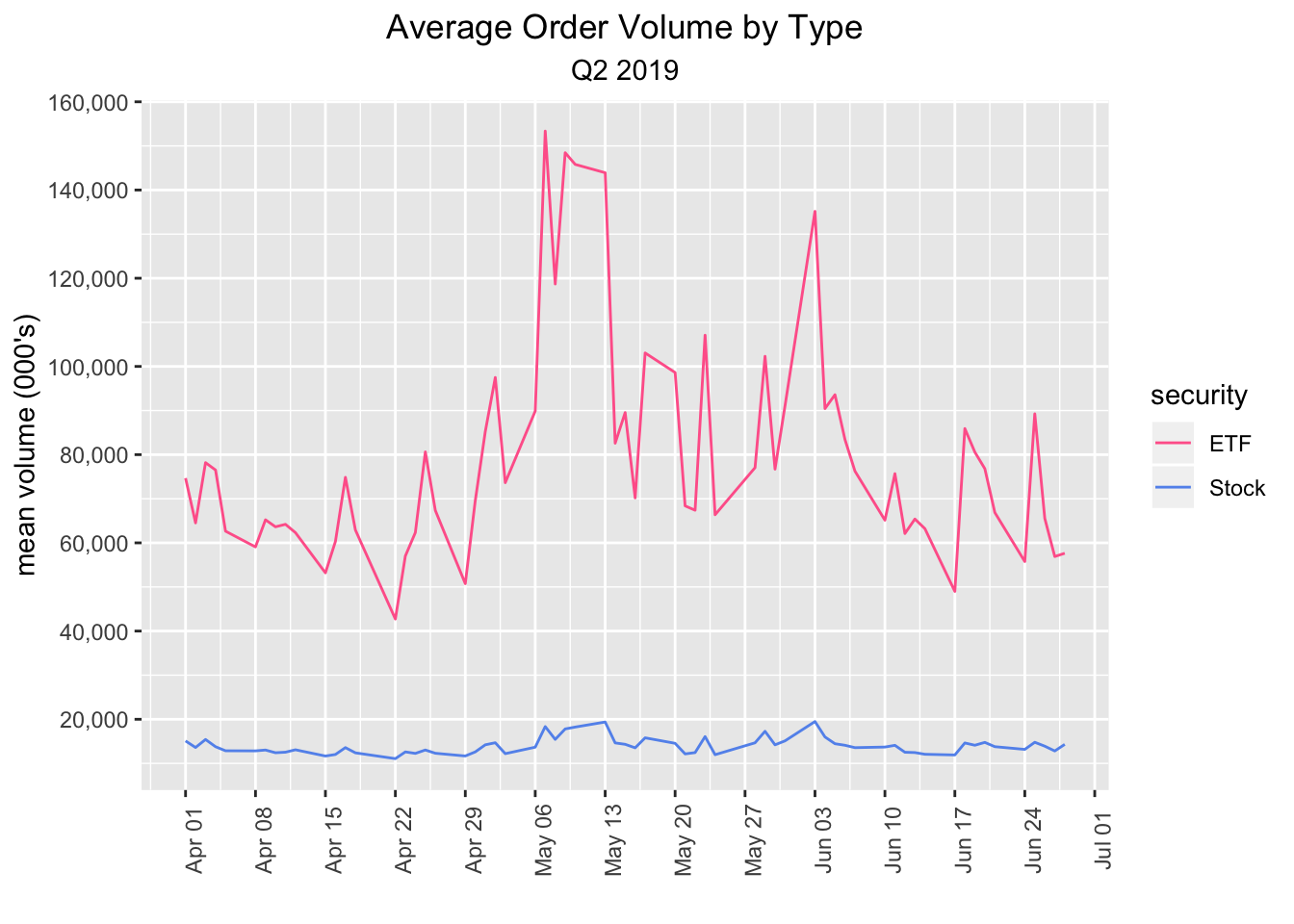
Well, we could keep exploring this data set and creating visualizations, and we will do so in the next post, but for now, let’s cover how to programatically import more data from the SEC.
Glance back up at our original import code flow and notice the only variables that we specified individually were year and quarter. That means we can create a function that accepts those two argumnents and then download data from the time period of our choice.
market_str_data_import <- function(year, quarter){


  market_structure_data_address <-
    paste0(
      "https://www.sec.gov/files/opa/data/market-structure/metrics-individual-security/individual_security_",
      year,
      "_",
      quarter,
      ".zip"
    )


  file_name <- paste0(quarter, "_", year, "_all.csv")

  temp <- tempfile()

  download.file(# location of file to be downloaded
    market_structure_data_address,
    # where we want R to store that file
    temp,
    mode = "wb",
    quiet = TRUE)


  vroom(unzip(temp, file_name)) %>%
    clean_names() %>%
    mutate(date = ymd(parse_date_time(date, "%Y%m%d")))

}
Let’s test the function on the third quarter of 2018
market_str_data_import("2018", "q3") %>%
  head()
# A tibble: 6 x 19
date security ticker mcap_rank turn_rank volatility_rank price_rank
<date> <chr> <chr> <dbl> <dbl> <dbl> <dbl>
1 2018-07-02 Stock A 10 5 1 9
2 2018-07-02 Stock AA 9 9 4 8
3 2018-07-02 Stock AAC 3 5 8 3
4 2018-07-02 Stock AAL 10 7 4 7
5 2018-07-02 Stock AAMC 2 2 10 9
6 2018-07-02 Stock AAME 2 1 10 2
# … with 12 more variables: lit_vol_000 <dbl>, order_vol_000 <dbl>,
# hidden <dbl>, trades_for_hidden <dbl>, hidden_vol_000 <dbl>,
# trade_vol_for_hidden_000 <dbl>, cancels <dbl>, lit_trades <dbl>,
# odd_lots <dbl>, trades_for_odd_lots <dbl>, odd_lot_vol_000 <dbl>,
# trade_vol_for_odd_lots_000 <dbl>If we wish to import data for all 4 quarters of a year, we can create a year_for_function variable to hold the years and a quarters_vector of quarters. We can then call map2_dfr() to loop over those quarters. For multiple years, we would create a vector years and loop over that as well.
year_for_function <- "2018"

quarters_vector <- c("q1", "q2", "q3", "q4")

market_structure_2018 <-
map2_dfr(year_for_function, quarters_vector, market_str_data_import)
Let’s start with the same count of stocks and ETFs
market_structure_2018 %>%
  group_by(security) %>%
  summarise(distinct_tickers = n_distinct(ticker))
# A tibble: 2 x 2
security distinct_tickers
<chr> <int>
1 ETF 2132
2 Stock 3928Same as before, we have 6060 tickers, broken down into 2132 ETFs and 3928 stocks, but now we have an entire year of daily observations.
Let’s grab one ticker, ‘TSLA’ and let’s also add another column called ‘day of the week’. We eventually want to visualize how certain market structure metrics are distributed across different trading days, so we need to convert from calendar dates to M-F.
ticker_chosen <- "TSLA"

market_structure_2018 %>%
  filter(ticker == ticker_chosen) %>%
  mutate(`day of the week` = as_factor(wday(date, label = TRUE, abbr = FALSE))) %>%
  select(date, `day of the week`, everything()) %>%
  head()
# A tibble: 6 x 20
date `day of the wee… security ticker mcap_rank turn_rank
<date> <ord> <chr> <chr> <dbl> <dbl>
1 2018-01-02 Tuesday Stock TSLA 10 10
2 2018-01-03 Wednesday Stock TSLA 10 10
3 2018-01-04 Thursday Stock TSLA 10 10
4 2018-01-05 Friday Stock TSLA 10 10
5 2018-01-08 Monday Stock TSLA 10 10
6 2018-01-09 Tuesday Stock TSLA 10 10
# … with 14 more variables: volatility_rank <dbl>, price_rank <dbl>,
# lit_vol_000 <dbl>, order_vol_000 <dbl>, hidden <dbl>,
# trades_for_hidden <dbl>, hidden_vol_000 <dbl>,
# trade_vol_for_hidden_000 <dbl>, cancels <dbl>, lit_trades <dbl>,
# odd_lots <dbl>, trades_for_odd_lots <dbl>, odd_lot_vol_000 <dbl>,
# trade_vol_for_odd_lots_000 <dbl>From here, we use ggplot to create density plots, faceted by day of the week.
ticker_chosen <- "TSLA"

market_structure_2018 %>%
  filter(ticker == ticker_chosen) %>%
  mutate(`day of the week` = as_factor(wday(date, label = TRUE, abbr = FALSE))) %>%
  select(date, `day of the week`, everything()) %>%
  ggplot(aes(x = order_vol_000)) +
  geom_density(aes(fill = `day of the week`), alpha = .3) +
  facet_grid(rows = vars(`day of the week`))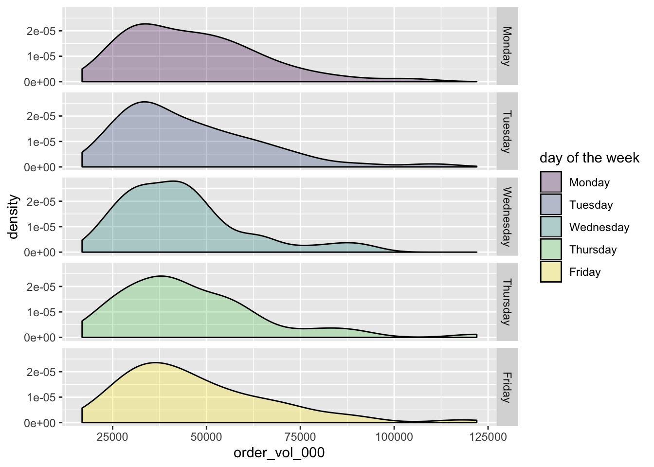
That looks pretty good, but let’s do some aesthetic cleanup. I don’t love that geom_density() includes the black line at the bottom. Let’s paint a white line over it with geom_hline(yintercept = 0, colour = "white", size = 1). We can add a title and caption with
labs(y = "", x = "", title = paste("2018 Order Volume Density for", ticker_chosen, sep = " "), caption = "source: SEC Midas").
Finally, order_vol_000 column is in the 000’s. Let’s clean up the x-axis labels with
scale_x_continuous(labels = function(l) {paste0(round(l / 1e6, 2), "B")}...).
ticker_chosen <- "TSLA"

market_structure_2018 %>%
  filter(ticker == ticker_chosen) %>%
  mutate(`day of the week` = as_factor(wday(date, label = TRUE, abbr = FALSE))) %>%
  select(date, `day of the week`, everything()) %>%
  ggplot(aes(x = order_vol_000)) +
  geom_density(aes(fill = `day of the week`), alpha = .3) +
  geom_hline(yintercept = 0,
             colour = "white",
             size = 1) +
  facet_grid(rows = vars(`day of the week`)) +
  labs(y = "", x = "",  title = paste("2018 Order Volume Density for", ticker_chosen, sep = " "), caption = "source: SEC Midas") +
  scale_x_continuous(
    labels = function(l) {paste0(round(l / 1e6, 2), "B")},
    breaks = scales::pretty_breaks(n = 10)
  ) +
   theme(plot.title = element_text(hjust = .5),
         plot.subtitle = element_text(hjust = .5))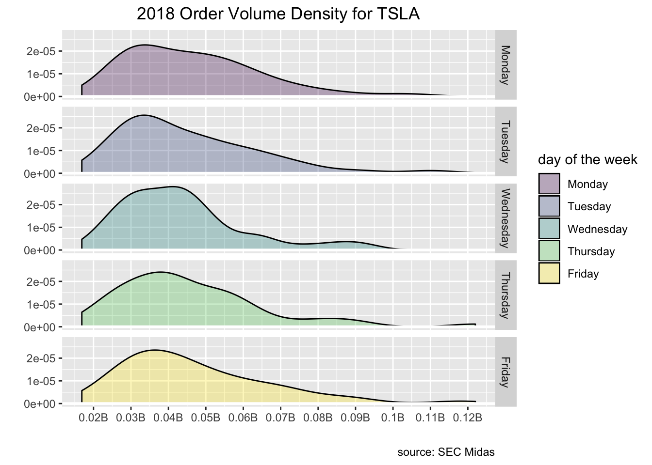
That’s all for today!
Shameless book plug for those who read to the end: if you like this sort of thing, check out my book Reproducible Finance with R!
Thanks for reading and see you next time.
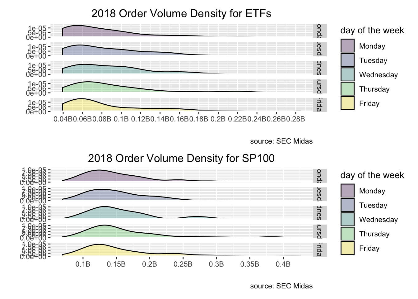
Here’s a quick addendum to this weekend’s post on order volume. Instead of comparing ETFs and stocks, let’s compare ETFs and just stocks in the SP100, i.e. probably the 100 stocks with the highest daily volume.
First, let’s get the tickers for the SP100. To do that, I’m going to import the tickers for OEF, Blackrock’s ETF that tracks the SP100. BLK is nice about making their fund holdings available so we can grab the tickers from this link: https://www.ishares.com/us/products/239723/ishares-sp-100-etf/1467271812596.ajax?fileType=csv&fileName=OEF_holdings&dataType=fund.
oef_sp100_holdings <- read_csv("https://www.ishares.com/us/products/239723/ishares-sp-100-etf/1467271812596.ajax?fileType=csv&fileName=OEF_holdings&dataType=fund",
    col_types = cols(ISIN = col_skip(), `Notional Value` = col_skip(),
        SEDOL = col_skip()), skip = 9) %>%
  mutate(fund = "oef",
         download_date = ymd(Sys.Date()))


oef_sp100_holdings %>%
  head()
# A tibble: 6 x 11
Ticker Name `Asset Class` `Weight (%)` Price Shares `Market Value`
<chr> <chr> <chr> <dbl> <dbl> <dbl> <dbl>
1 AAPL APPL… Equity 7.41 310. 1.38e6 426849725.
2 MSFT MICR… Equity 7.09 162. 2.52e6 408162395.
3 AMZN AMAZ… Equity 4.54 1901. 1.37e5 261333541.
4 FB FACE… Equity 3.01 218. 7.94e5 173402676.
5 BRKB BERK… Equity 2.56 229. 6.46e5 147626272.
6 JPM JPMO… Equity 2.47 137. 1.04e6 142284210.
# … with 4 more variables: Sector <chr>, Exchange <chr>, fund <chr>,
# download_date <date>We have a wealth of information in this data frame but we need only the tickers so that we can filter our original Midas data set down to stocks in the SP100.
oef_sp100_tickers <-
oef_sp100_holdings %>%
  clean_names() %>%
  select(ticker, sector, asset_class) %>%
  mutate(ticker = str_replace(ticker, "BRKB", "BRK.B")) %>%
  filter(asset_class == "Equity") %>%
  pull(ticker)
Now that we have the tickers for the SP100, we can filter our original data down to just ETFs and stock tickers that match the vector oef_sp100_tickers.
market_structure_2018_etfs_sp100 <-
market_structure_2018 %>%
  filter(security == "ETF" | ticker %in% oef_sp100_tickers)

market_structure_2018_etfs_sp100 %>%
  group_by(security) %>%
  summarise(distinct_tickers = n_distinct(ticker))
# A tibble: 2 x 2
security distinct_tickers
<chr> <int>
1 ETF 2132
2 Stock 94We matched on only 94 of the 101. Not a huge deal for today’s purposes but let’s figure out which ones did not match.
setdiff(oef_sp100_tickers, market_structure_2018_etfs_sp100$ticker)[1] "MDT" "ACN" "AGN" "SLB" "DD" "SPG" "DOW"Well, MDT pops out a bit, that’s Medtronic. Probably worth investigating why we can’t locate that ticker in the Midas/SEC data, for now, though, we’ll plow on to some visualizations.
market_structure_2018_etfs_sp100 %>%
  select(date, security, ticker, order_vol_000) %>%
  mutate(security = case_when(security == "Stock" ~ "SP100",
                              TRUE ~ "ETF")) %>%
  group_by(security, date) %>%
  summarise(mean_vol = mean(order_vol_000)) %>%
  ggplot(aes(x = date, y = mean_vol, color = security)) +
    geom_line() +
  scale_x_date(breaks = scales::pretty_breaks(n = 20)) +
  scale_y_continuous(label = scales::comma_format(), breaks = scales::pretty_breaks(n = 10)) +
  theme(axis.text.x = element_text(angle = 90),
        plot.title = element_text(hjust = .5),
        plot.subtitle = element_text(hjust = .5)) +
  labs(x = "", y = "mean volume (000's)", title = "Average Order Volume by Type", subtitle = "Q2 2019") +
  scale_colour_manual(values = c("#ff6699", "cornflowerblue"))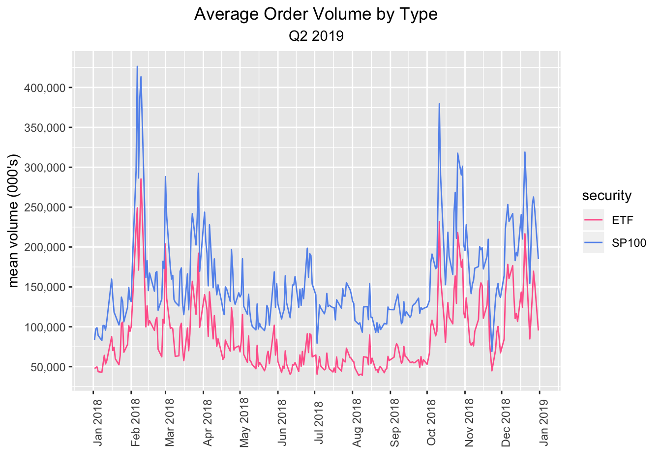
etf_plot <-
market_structure_2018_etfs_sp100 %>%
  group_by(security, date) %>%
  summarise(mean_vol = mean(order_vol_000)) %>%
  mutate(`day of the week` = as_factor(wday(date, label = TRUE, abbr = FALSE))) %>%
  filter(security == "ETF") %>%
  select(date, `day of the week`, everything()) %>%
  ggplot(aes(x = mean_vol)) +
  geom_density(aes(fill = `day of the week`), alpha = .3) +
  geom_hline(yintercept = 0,
             colour = "white",
             size = 1) +
  facet_grid(rows = vars(`day of the week`)) +
  labs(y = "", x = "",  title = "2018 Order Volume Density for ETFs", caption = "source: SEC Midas") +
  scale_x_continuous(
    labels = function(l) {paste0(round(l / 1e6, 2), "B")},
    breaks = scales::pretty_breaks(n = 10)
  ) +
   theme(plot.title = element_text(hjust = .5),
         plot.subtitle = element_text(hjust = .5))

etf_plot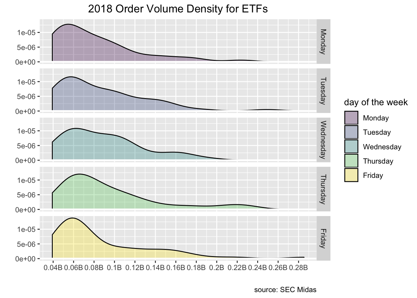
sp100_plot <- market_structure_2018_etfs_sp100 %>%
  select(date, security, ticker, order_vol_000) %>%
  mutate(security = case_when(security == "Stock" ~ "SP100",
                              TRUE ~ "ETF")) %>%
  group_by(security, date) %>%
  summarise(mean_vol = mean(order_vol_000)) %>%
  mutate(`day of the week` = as_factor(wday(date, label = TRUE, abbr = FALSE))) %>%
  filter(security == "SP100") %>%
  select(date, `day of the week`, everything()) %>%
  ggplot(aes(x = mean_vol)) +
  geom_density(aes(fill = `day of the week`), alpha = .3) +
  geom_hline(yintercept = 0,
             colour = "white",
             size = 1) +
  facet_grid(rows = vars(`day of the week`)) +
  labs(y = "", x = "",  title = "2018 Order Volume Density for SP100", caption = "source: SEC Midas") +
  scale_x_continuous(
    labels = function(l) {paste0(round(l / 1e6, 2), "B")},
    breaks = scales::pretty_breaks(n = 10)
  ) +
   theme(plot.title = element_text(hjust = .5),
         plot.subtitle = element_text(hjust = .5))

sp100_plot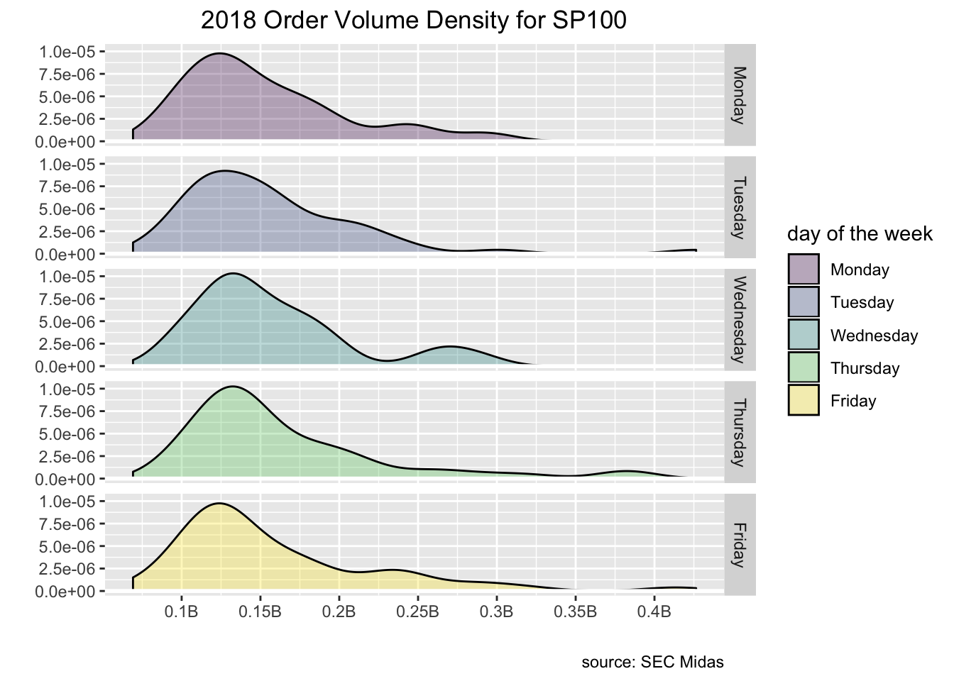
library(patchwork)

etf_plot / sp100_plot