The Sortino Ratio is similar to the Sharpe Ratio except that the riskiness of a portfolio is measured by the deviation of returns below a target return, instead of by the standard deviation of all returns. This stands in contradistinction to the Sharpe Ratio, which measures return/risk by the ratio of the returns above the risk free rate divided by the standard deviation of all returns. By way of history, Harry Markowitz, Nobel laureate and father of MPT whom we mentioned in this section’s introduction, noted that downside deviation might be a better measure of risk than the standard deviation of all returns, but its calculation was computationally too expensive1 (it was 1959, if he only he’d had R on his laptop).
The Sortino Ratio equation is as follows:
\[Sortino~Ratio_{portfolio}=\frac{(\overline{Return_{portfolio}-MAR})}{\sqrt{\sum_{t=1}^n min(R_t-MAR,~0)^2}/n}\]
The denominator in that equation (called the Downside Deviation, semi-deviation or downside risk) can be thought of as the deviation of the returns that fall below some target rate of return for the portfolio. That target rate is called the Minimum Acceptable Rate, or MAR. The numerator is the mean portfolio return minus the MAR. It can be thought of as excess returns in the same was as the numerator of the Sharpe Ratio, except for Sortino it’s in excess of whatever minimum rate our team (or our clients) choose.
Let’s assign the MAR of .8% to the variable MAR. Note that we are holding this portfolio to a higher standard now than we did in the last chapter.
MAR <- .0008Just as we reused a lot of our skewness code flow in our kurtosis calculation, we will reuse some Sharpe code flow for the Sortino calculations.
Calculating Sortino Ratio in the xts world
In the xts world, very similar to the Sharpe Ratio, PerformanceAnalytics makes it quick to calculate Sortino. It’s the same code as we used for Sharpe, except we call the function SortinoRatio() instead of SharpeRatio(), and the argument is MAR = MAR instead of Rf = rfr.
sortino_xts <-
  SortinoRatio(portfolio_returns_xts_rebalanced_monthly,
               MAR = MAR) %>%
  `colnames<-`("ratio")
Calculating Sortino Ratio in the tidyverse
Next we head to dplyr and run a by-hand calculation with summarise(ratio = mean(returns - MAR)/sqrt(sum(pmin(returns - MAR, 0)^2)/nrow(.))). This should look familiar from the previous chapter, but with a different equation.
sortino_byhand <-
  portfolio_returns_tq_rebalanced_monthly %>%
  summarise(ratio = mean(returns - MAR)/
              sqrt(sum(pmin(returns - MAR, 0)^2)/
                     nrow(.)))
Calculating Sortino Ratio in the tidyquant world
Now on to tidyquant, which allows us to apply the SortinoRatio() function from PerformanceAnalytics to a tibble.
sortino_tidy <-
  portfolio_returns_tq_rebalanced_monthly %>%
  tq_performance(Ra = returns,
                 performance_fun = SortinoRatio,
                 MAR = MAR,
                 method = "full") %>%
  `colnames<-`("ratio")
Let’s compare our 3 Sortino objects.
sortino_tidy %>%
  mutate(sortino_byhand = sortino_byhand$ratio,
         sortino_xts = sortino_xts[1])
## # A tibble: 1 x 3
## ratio sortino_byhand sortino_xts
## <dbl> <dbl> <dbl>
## 1 0.422 0.422 0.445We have consistent results from xts, tidyquant and our by-hand piped calculation. Again, the Sortino Ratio is most informative when compared to other Sortino Ratios. Is our portfolio’s Sortino good, great, awful? We can compare to the Sortino Ratio of the S&P500 in the same time period.
market_returns_sortino <-
  market_returns_tidy %>%
  summarise(ratio = mean(returns - MAR)/
              sqrt(sum(pmin(returns - MAR, 0)^2)/
                     nrow(.)))

market_returns_sortino$ratio
## [1] 0.7765608The S&P500 has beat our portfolio again. That makes some sense given that the S&P500 also had a higher Sharpe Ratio.
Visualizing the Sortino Ratio
Very similar to our work on the Sharpe Ratio, we will add a column for returns that fall below MAR with mutate(returns_below_MAR = ifelse(returns < MAR, returns, NA)) and add a column for returns above MAR with mutate(returns_above_MAR = ifelse(returns > MAR, returns, NA)). We do this with an eye towards ggplot.
sortino_byhand <-
  portfolio_returns_tq_rebalanced_monthly %>%
  mutate(ratio = mean(returns - MAR)/
           sqrt(sum(pmin(returns - MAR, 0)^2)/
                  nrow(.))) %>%
  mutate(returns_below_MAR =
           if_else(returns < MAR, returns, as.numeric(NA))) %>%
  mutate(returns_above_MAR =
           if_else(returns > MAR, returns, as.numeric(NA)))
We use that new object with new columns to create a scatterplot of returns using ggplot. again to grasp how many of our returns are above the MAR and how many are below the MAR.
sortino_byhand %>%
  ggplot(aes(x = date)) +
  geom_point(aes(y = returns_below_MAR),
             colour = "red") +
  geom_point(aes(y = returns_above_MAR),
             colour = "green") +
  geom_vline(xintercept = as.numeric(as.Date("2016-11-30")),
             color = "blue") +
  geom_hline(yintercept = MAR, color = "purple",
             linetype = "dotted") +
  annotate(geom="text", x=as.Date("2016-11-30"),
           y = -.05,
           label = "Election",
           fontface = "plain",
           angle = 90,
           alpha = .5,
           vjust =  1.5) +
  ylab("percent monthly returns")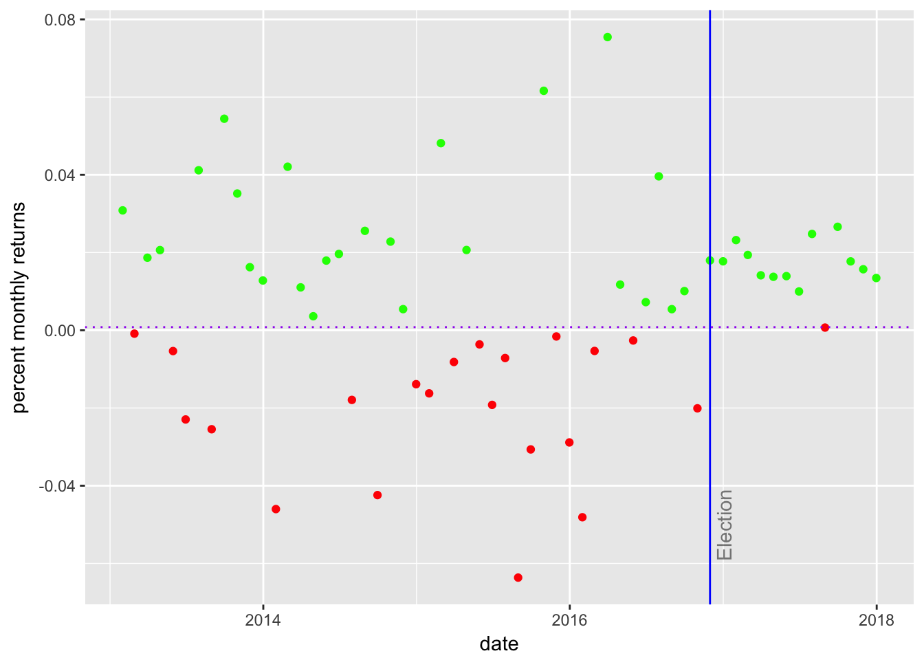
Figure 1: Scatter Returns with MAR
Histogram of Returns with MAR
sortino_byhand %>%
  ggplot(aes(x = returns)) +
  geom_histogram(alpha = 0.25,
                 binwidth = .01,
                 fill = "cornflowerblue") +
  geom_vline(xintercept = MAR,
             color = "green") +
  annotate(geom = "text",
           x = MAR,
           y = 13,
           label = "MAR",
           fontface = "plain",
           angle = 90,
           alpha = .5,
           vjust =  1)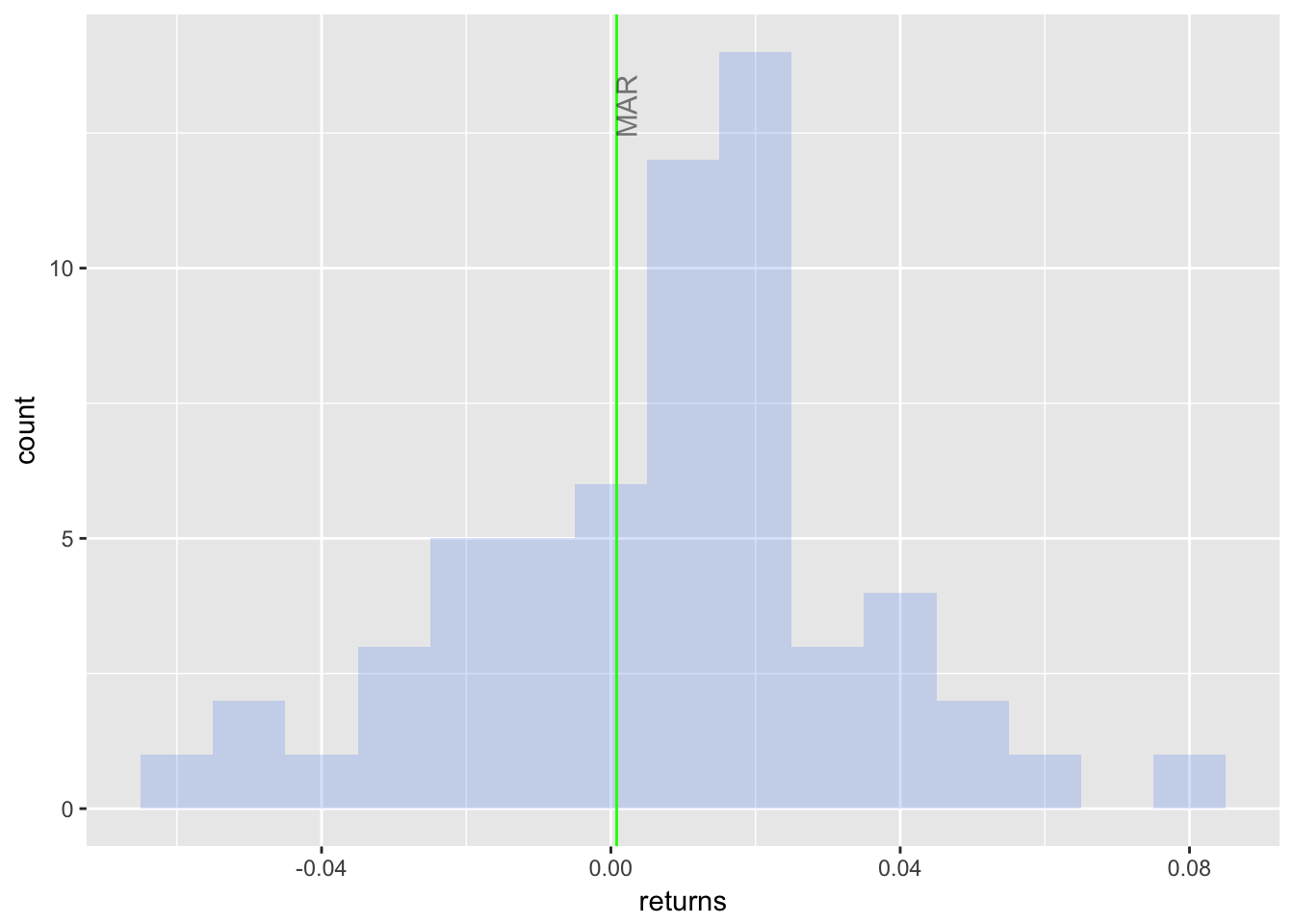
Figure 2: Histogram Returns with MAR
Density Plot
sortino_density_plot <-
  sortino_byhand %>%
  ggplot(aes(x = returns)) +
  stat_density(geom = "line", size = 1, color = "cornflowerblue")

shaded_area_data <- ggplot_build(sortino_density_plot)$data[[1]] %>%
  filter(x < MAR)

sortino_density_plot_shaded <- sortino_density_plot +
  geom_area(data = shaded_area_data, aes(x = x, y = y), fill="pink", alpha = 0.5)

sortino_density_plot_shaded +
  geom_segment(aes(x = 0,
                   y = 1.5,
                   xend = -.05,
                   yend = 1.5),
  arrow = arrow(length = unit(0.4, "cm")),
  size = .05) +
  geom_segment(data = shaded_area_data,
               aes(x = MAR, y = 0, xend = MAR, yend = y),
               color = "red",
               linetype = "dotted") +
  annotate(geom = "text",
           x = MAR,
           y = 5,
           label = "MAR = 0.8%",
           fontface = "plain",
           angle = 90,
           alpha = .8,
           vjust =  -1) +
  annotate(geom = "text",
           x = -.02,
           y = .1,
           label = "Downside",
           fontface = "plain",
           alpha = .8,
           vjust =  -1)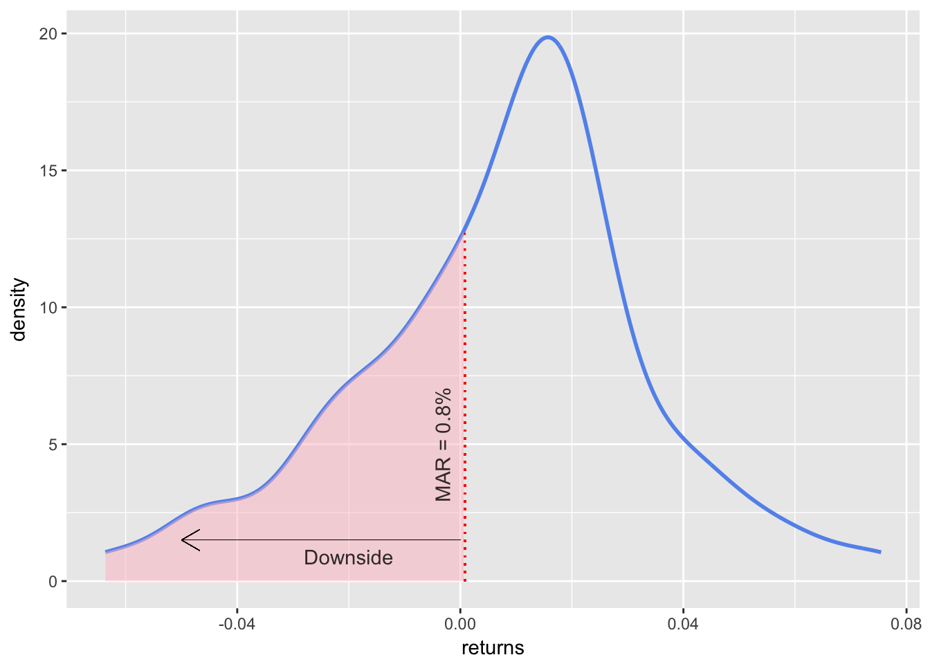
Figure 3: Density for Sortino
Rolling Sortino Ratio with in the xts World
We will calculate the rolling 24-month Sortino on the idea that 24-months is a sufficiently large window for our denominator. Our code flow is very similar that of the Sharpe Ratio.
window <- 24

rolling_sortino_xts <-
  rollapply(portfolio_returns_xts_rebalanced_monthly,
            window,
            function(x)
            SortinoRatio(x, MAR = MAR)) %>%
  na.omit() %>%
  `colnames<-`("sortino")
Rolling Sortino Ratio with in tidyverse + tibbletime
Similar to what we did with the Sharpe Ratio, we can combine the tidyverse and tibbletime by we are going to writing our own function with rollify().
sortino_roll_24 <- rollify(function(returns) {
    ratio = mean(returns - MAR)/
      sqrt(sum(pmin(returns - MAR, 0)^2)/
             length(returns))
    },
window = 24)


rolling_sortino_tidy_tibbletime <-
  portfolio_returns_tq_rebalanced_monthly %>%
  as_tbl_time(index = date) %>%
  mutate(ratio = sortino_roll_24(returns)) %>%
  na.omit() %>%
  select(-returns)
Rolling Sortino Ratio using Tidyquant
To calculate the rolling Sharpe Ration using tidyquant and the built-in SortinoRatio() function, we first build our own, custom function where we can specify the RFR and an argument to the SortinoRatio() function
sortino_tq_roll <- function(df){
  SortinoRatio(df, MAR = MAR)
}
rolling_sortino_tq <-
portfolio_returns_tq_rebalanced_monthly %>%
tq_mutate(
select = returns,
mutate_fun = rollapply,
width = window,
align = "right",
FUN = sortino_tq_roll,
col_rename = "Sortino"
) %>%
na.omit()Now we can compare our 3 rolling Sharpe Ratio objects and confirm consistency.
rolling_sortino_tidy_tibbletime %>%
  mutate(sortino_xts = coredata(rolling_sortino_xts),
         sortino_tq = rolling_sortino_tq$Sortino) %>%
  na.omit() %>%
  head()
## # A time tibble: 6 x 4
## # Index: date
## date ratio sortino_xts sortino_tq
## <date> <dbl> <dbl> <dbl>
## 1 2014-12-31 0.488 0.537 0.488
## 2 2015-01-31 0.355 0.385 0.355
## 3 2015-02-28 0.482 0.516 0.482
## 4 2015-03-31 0.409 0.443 0.409
## 5 2015-04-30 0.410 0.432 0.410
## 6 2015-05-31 0.415 0.441 0.415Visualizing the Sortino Ratio
We will again start with highcharter and pass in our rolling_sortino_xts
highchart(type = "stock") %>%
  hc_title(text = "Rolling Sortino") %>%
  hc_add_series(rolling_sortino_xts,
                name = "Sortino",
                color = "cornflowerblue") %>%
  hc_navigator(enabled = FALSE) %>%
  hc_scrollbar(enabled = FALSE) %>%
  hc_add_theme(hc_theme_flat()) %>%
  hc_exporting(enabled = TRUE)
I am not going to port this rolling Sortino to ggplot and the tidyverse, but it would follow the exact same code flow as we used for the Sharpe Ratio.
Have a look here.
Shiny Sortino Ratio
We now port this Sortino work into a Shiny app - and notice how similar it is to the Sharpe Ratio app in structure.
Here is the link.
Markowitz, Harry. Portfolio Selection: Efficient Diversification of Investments, John Wiley & Sons, 1959↩