A note to all readers
A recent release of ggplot2 and rlang caused some issues with highcharter version 0.5.0. The next release on CRAN, to version 0.6.0, will fix the issues. Until then, you’ll need the development version of highcharter to run the code in this chapter.
devtools::install_github("jbkunst/highcharter")
library(highcharter)
Monte Carlo Simulation
mean_port_return <-
  mean(portfolio_returns_tq_rebalanced_monthly$returns)

stddev_port_return <-
  sd(portfolio_returns_tq_rebalanced_monthly$returns)
simulated_monthly_returns <- rnorm(120,
mean_port_return,
stddev_port_return)head(simulated_monthly_returns)## [1] 0.076073166 0.001458752 0.025330084 0.021832285 0.019757856 0.013746874tail(simulated_monthly_returns)## [1] 0.029984301 -0.046513503 0.027205829 0.041044671 -0.008972907
## [6] -0.033927739simulated_returns_add_1 <-
tibble(c(1, 1 + simulated_monthly_returns)) %>%
`colnames<-`("returns")
head(simulated_returns_add_1)## # A tibble: 6 x 1
## returns
## <dbl>
## 1 1
## 2 1.08
## 3 1.00
## 4 1.03
## 5 1.02
## 6 1.02simulated_growth <-
simulated_returns_add_1 %>%
mutate(growth1 = accumulate(returns, function(x, y) x * y),
growth2 = accumulate(returns, `*`),
growth3 = cumprod(returns)) %>%
dplyr::select(-returns)
tail(simulated_growth)## # A tibble: 6 x 3
## growth1 growth2 growth3
## <dbl> <dbl> <dbl>
## 1 3.05 3.05 3.05
## 2 2.91 2.91 2.91
## 3 2.99 2.99 2.99
## 4 3.11 3.11 3.11
## 5 3.08 3.08 3.08
## 6 2.98 2.98 2.98cagr <-
((simulated_growth$growth1[nrow(simulated_growth)]^
(1/10)) -1)*100Several Simulation Functions
simulation_accum_1 <- function(init_value, N, mean, stdev) {
    tibble(c(init_value, 1 + rnorm(N, mean, stdev))) %>%
    `colnames<-`("returns") %>%
    mutate(growth =
             accumulate(returns,
                        function(x, y) x * y)) %>%
    dplyr::select(growth)
}
simulation_accum_2 <- function(init_value, N, mean, stdev) {
tibble(c(init_value, 1 + rnorm(N, mean, stdev))) %>%
`colnames<-`("returns") %>%
mutate(growth = accumulate(returns, `*`)) %>%
dplyr::select(growth)
}simulation_cumprod <- function(init_value, N, mean, stdev) {
tibble(c(init_value, 1 + rnorm(N, mean, stdev))) %>%
`colnames<-`("returns") %>%
mutate(growth = cumprod(returns)) %>%
dplyr::select(growth)
}simulation_confirm_all <- function(init_value, N, mean, stdev) {
tibble(c(init_value, 1 + rnorm(N, mean, stdev))) %>%
`colnames<-`("returns") %>%
mutate(growth1 = accumulate(returns, function(x, y) x * y),
growth2 = accumulate(returns, `*`),
growth3 = cumprod(returns)) %>%
dplyr::select(-returns)
}simulation_confirm_all_test <-
simulation_confirm_all(1, 120,
mean_port_return, stddev_port_return)
tail(simulation_confirm_all_test)## # A tibble: 6 x 3
## growth1 growth2 growth3
## <dbl> <dbl> <dbl>
## 1 2.80 2.80 2.80
## 2 2.82 2.82 2.82
## 3 2.91 2.91 2.91
## 4 2.84 2.84 2.84
## 5 2.94 2.94 2.94
## 6 2.96 2.96 2.96Running Multiple Simulations
sims <- 51
starts <-
  rep(1, sims) %>%
set_names(paste("sim", 1:sims, sep = ""))head(starts)## sim1 sim2 sim3 sim4 sim5 sim6
## 1 1 1 1 1 1tail(starts)## sim46 sim47 sim48 sim49 sim50 sim51
## 1 1 1 1 1 1monte_carlo_sim_51 <-
map_dfc(starts, simulation_accum_1,
N = 120,
mean = mean_port_return,
stdev = stddev_port_return)
tail(monte_carlo_sim_51 %>% dplyr::select(growth1, growth2,
growth49, growth50), 3)## # A tibble: 3 x 4
## growth1 growth2 growth49 growth50
## <dbl> <dbl> <dbl> <dbl>
## 1 2.27 2.09 3.11 4.13
## 2 2.20 2.14 3.14 4.23
## 3 2.19 2.19 3.19 4.39monte_carlo_sim_51 <-
monte_carlo_sim_51 %>%
mutate(month = seq(1:nrow(.))) %>%
dplyr::select(month, everything()) %>%
`colnames<-`(c("month", names(starts))) %>%
mutate_all(funs(round(., 2)))
tail(monte_carlo_sim_51 %>% dplyr::select(month, sim1, sim2,
sim49, sim50), 3)## # A tibble: 3 x 5
## month sim1 sim2 sim49 sim50
## <dbl> <dbl> <dbl> <dbl> <dbl>
## 1 119 2.26 2.27 2.08 3.11
## 2 120 2.33 2.2 2.06 3.14
## 3 121 2.23 2.19 2.19 3.19monte_carlo_rerun_5 <-
rerun(.n = 5,
simulation_accum_1(1,
120,
mean_port_return,
stddev_port_return))map(monte_carlo_rerun_5, head)## [[1]]
## # A tibble: 6 x 1
## growth
## <dbl>
## 1 1
## 2 0.995
## 3 1.01
## 4 1.03
## 5 1.03
## 6 1.06
##
## [[2]]
## # A tibble: 6 x 1
## growth
## <dbl>
## 1 1
## 2 1.01
## 3 1.01
## 4 1.02
## 5 0.998
## 6 1.00
##
## [[3]]
## # A tibble: 6 x 1
## growth
## <dbl>
## 1 1
## 2 1.01
## 3 1.02
## 4 1.05
## 5 1.05
## 6 1.04
##
## [[4]]
## # A tibble: 6 x 1
## growth
## <dbl>
## 1 1
## 2 1.04
## 3 1.03
## 4 1.05
## 5 1.02
## 6 0.996
##
## [[5]]
## # A tibble: 6 x 1
## growth
## <dbl>
## 1 1
## 2 1.01
## 3 1.04
## 4 1.04
## 5 1.02
## 6 1.01reruns <- 51
monte_carlo_rerun_51 <-
rerun(.n = reruns,
simulation_accum_1(1,
120,
mean_port_return,
stddev_port_return)) %>%
simplify_all() %>%
`names<-`(paste("sim", 1:reruns, sep = " ")) %>%
as_tibble() %>%
mutate(month = seq(1:nrow(.))) %>%
dplyr::select(month, everything())
monte_carlo_rerun_51 %>%
select(`sim 1`, `sim 2`,`sim 49`, `sim 50`) %>%
tail(3)## # A tibble: 3 x 4
## `sim 1` `sim 2` `sim 49` `sim 50`
## <dbl> <dbl> <dbl> <dbl>
## 1 2.76 2.15 2.10 1.77
## 2 2.66 2.13 2.14 1.72
## 3 2.70 2.20 2.18 1.74Visualizing Simulation Results
monte_carlo_sim_51 %>%
  gather(sim, growth, -month) %>%
  group_by(sim) %>%
  ggplot(aes(x = month, y = growth, color = sim)) +
  geom_line() +
  theme(legend.position="none")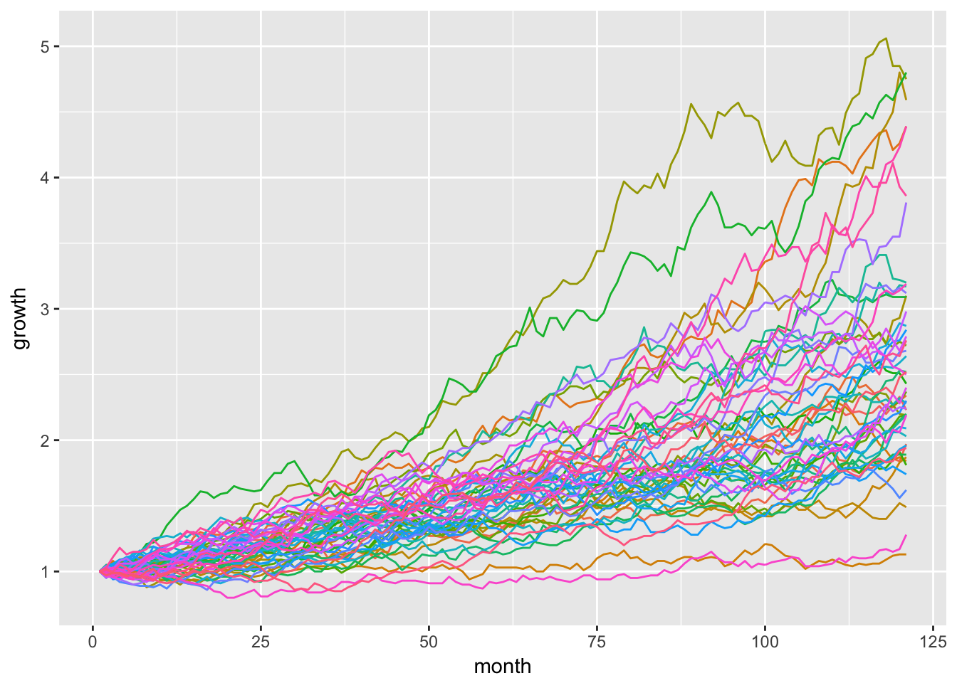
Figure 1: 51 Simulations ggplot
sim_summary <-
monte_carlo_sim_51 %>%
  gather(sim, growth, -month) %>%
  group_by(sim) %>%
  summarise(final = last(growth)) %>%
  summarise(
            max = max(final),
            min = min(final),
            median = median(final))
sim_summary
## # A tibble: 1 x 3
## max min median
## <dbl> <dbl> <dbl>
## 1 4.8 1.13 2.4monte_carlo_sim_51 %>%
gather(sim, growth, -month) %>%
group_by(sim) %>%
filter(
last(growth) == sim_summary$max ||
last(growth) == sim_summary$median ||
last(growth) == sim_summary$min) %>%
ggplot(aes(x = month, y = growth)) +
geom_line(aes(color = sim)) 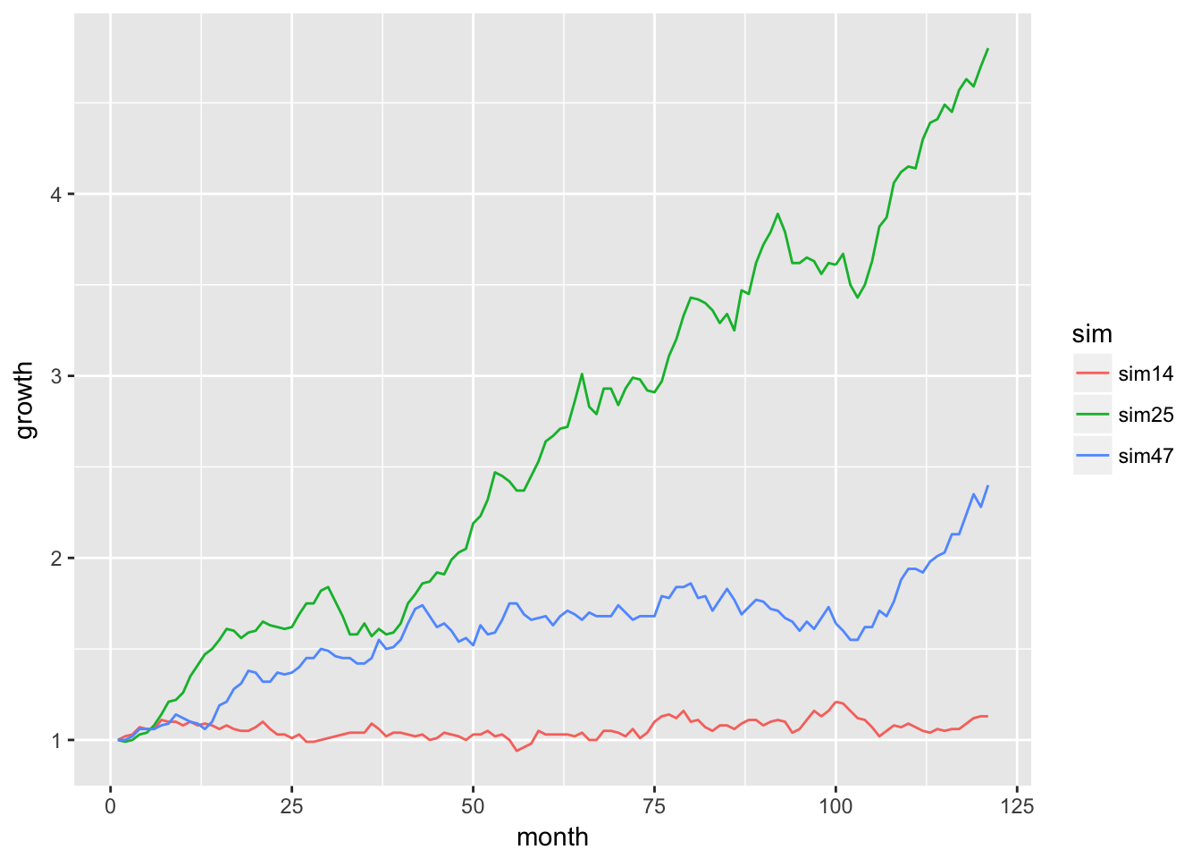
Figure 2: Min, Max, Median Sims ggplot
probs <- c(.005, .025, .25, .5, .75, .975, .995)sim_final_quantile <-
monte_carlo_sim_51 %>%
gather(sim, growth, -month) %>%
group_by(sim) %>%
summarise(final = last(growth))quantiles <-
quantile(sim_final_quantile$final, probs = probs) %>%
tibble() %>%
`colnames<-`("value") %>%
mutate(probs = probs) %>%
spread(probs, value)
quantiles[, 1:6]## # A tibble: 1 x 6
## `0.005` `0.025` `0.25` `0.5` `0.75` `0.975`
## <dbl> <dbl> <dbl> <dbl> <dbl> <dbl>
## 1 1.17 1.33 2.06 2.4 3.04 4.71Visualizing with highcharter
mc_gathered <-
  monte_carlo_sim_51 %>%
  gather(sim, growth, -month) %>%
  group_by(sim)
# This takes a few seconds to run
hchart(mc_gathered,
type = 'line',
hcaes(y = growth,
x = month,
group = sim)) %>%
hc_title(text = "51 Simulations") %>%
hc_xAxis(title = list(text = "months")) %>%
hc_yAxis(title = list(text = "dollar growth"),
labels = list(format = "${value}")) %>%
hc_add_theme(hc_theme_flat()) %>%
hc_exporting(enabled = TRUE) %>%
hc_legend(enabled = FALSE)mc_max_med_min <-
mc_gathered %>%
filter(
last(growth) == sim_summary$max ||
last(growth) == sim_summary$median ||
last(growth) == sim_summary$min) %>%
group_by(sim)hchart(mc_max_med_min,
type = 'line',
hcaes(y = growth,
x = month,
group = sim)) %>%
hc_title(text = "Min, Max, Median Simulations") %>%
hc_xAxis(title = list(text = "months")) %>%
hc_yAxis(title = list(text = "dollar growth"),
labels = list(format = "${value}")) %>%
hc_add_theme(hc_theme_flat()) %>%
hc_exporting(enabled = TRUE) %>%
hc_legend(enabled = FALSE)