Today we’ll explore the relationship between the VIX and the past, realized volatility of the S&P 500.
The VIX is a measure of the expected future volatility of the S&P500 and it has been quite low recently. As a volatility nerd, I came across an interesting piece from AQR on the meaning of the VIX. As a reproducibility and R nerd, I decided to reproduce some of the findings using R. Obviously, the substance and ideas here are 100% attributable to AQR. My goal is add to our R volatility toolbox and engage with that interesting AQR post - for me, an effective way to understand new research is to reproduce it.
With that said, let’s get started.
First we’ll need the price histories of the S&P500 and the VIX, and we’ll convert S&P500 prices to returns.
symbols <- c("^GSPC", "^VIX")

prices<-
  getSymbols(symbols, src = 'yahoo', from = "1990-01-01",
             auto.assign = TRUE, warnings = FALSE) %>%
  map(~Cl(get(.)))

# get daily, cont compounded returns
sp500_returns <- na.omit(ROC(GSPC$GSPC.Close, 1, type = "continuous"))
Now we need to calculate the 20-day and 60-day trailing volatility of the S&P500 returns and annualize that volatility. We will use rollapply and the StdDev() function for the initial calculation, and then will annualize assuming 252 trading days in a year.
sp500_rolling_sd_20 <- rollapply(sp500_returns,
                             20,
                             function(x) StdDev(x))

sp500_rolling_sd_60 <- rollapply(sp500_returns,
                             60,
                             function(x) StdDev(x))

sp500_rolling_sd_annualized_20 <- (round((sqrt(252) * sp500_rolling_sd_20 * 100), 2))
sp500_rolling_sd_annualized_60 <- (round((sqrt(252) * sp500_rolling_sd_60 * 100), 2))
Now we have the VIX price history and the rolling 20-day and 60-day volatility of S&P500 returns, annualized. Let’s merge them to one xts object using merge.xts().
vol_vix_xts <- merge.xts(VIX$VIX.Close, sp500_rolling_sd_annualized_20, sp500_rolling_sd_annualized_60)If we were going to use highcharter for our visualizations, we could stop here but now seems like a good time to explore ggplot2 so we will convert that xts object to a tibble. We’ll use the as_tibble() function from the tidyquant package and set preserve_row_names = TRUE.
vol_vix_df <-
  vol_vix_xts %>%
  as_tibble(preserve_row_names = TRUE) %>%
  mutate(date = ymd(row.names)) %>%
  select(date, everything(), -row.names) %>%
  rename(vix = VIX.Close, realized_vol_20 = GSPC.Close, realized_vol_60 = GSPC.Close.1)
Let’s start with a scatterplot to show 20-day trailing volatility on the x-axis and the VIX on the y-axis. Now that our data is in a tibble, it’s a straightforward ggplot2 call, though we’ll add some aesthetic cleanup of axis labels to keep things interesting.
ggplot_trailing20 <-
  ggplot(vol_vix_df, aes(realized_vol_20, vix)) +
  geom_point(colour = "light blue") +
  geom_smooth(method='lm', se = FALSE, color = "pink", size = .5) +
  ggtitle("Vix versus 20-Day Realized Vol") +
  xlab("Realized vol preceding 20 trading days") +
  ylab("Vix") +
  # Add a '%' sign to the axes without having to rescale.
  scale_y_continuous(labels = function(x){ paste0(x, "%") }) +
  scale_x_continuous(labels = function(x){ paste0(x, "%") }) +
  theme(plot.title = element_text(hjust = 0.5))

ggplot_trailing20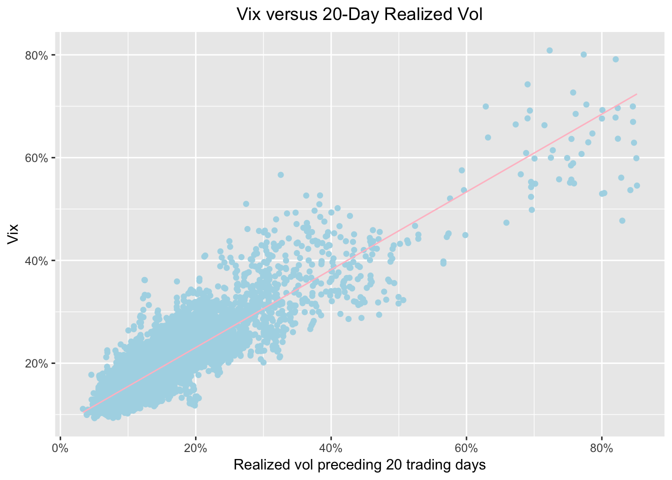
The scatterplot seems to be showing that the VIX is reflective of recent realized market volatility, and perhaps not telling us much more than that. That may or may not sound earth shattering but it emphasizes that when people talk about the VIX being very low, they are saying recent volatility has been very low.
Again, a deeper look at the substance can found in the original post by AQR and if any VIX experts disagree with the inferences being drawn here, I am happy to be enlightened.
Let’s take a look at a scatter with trailing 60-day volatility on the x-axis.
ggplot_trailing60 <-
  ggplot(vol_vix_df, aes(realized_vol_60, vix)) +
  geom_point(colour = "blue") +
  geom_smooth(method='lm', se = FALSE, color = "red", size = .5) +
  ggtitle("Vix versus 60-Day Realized Vol") +
  xlab("Realized vol preceding 60 trading days") +
  ylab("Vix") +
  scale_y_continuous(labels = function(x){ paste0(x, "%") }) +
  scale_x_continuous(labels = function(x){ paste0(x, "%") }) +
  theme(plot.title = element_text(hjust = 0.5))

ggplot_trailing60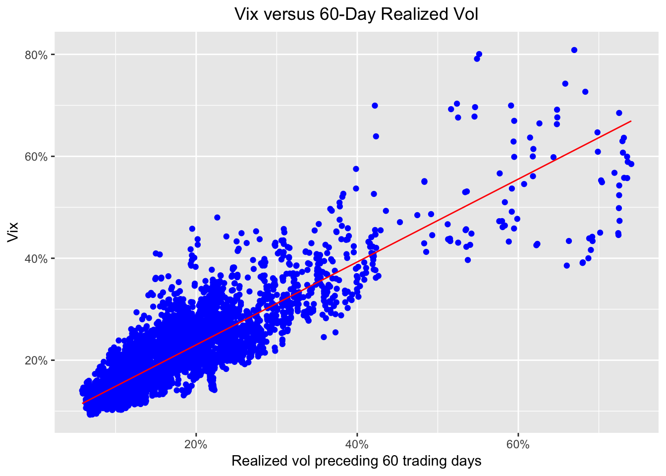
Those two scatterplots look similar, implying that trailing 20-day and trailing 60-day realized volatility are both good explainers of the VIX. Instead of relying on our eyeballs, though, let’s reproduce AQR’s statistics with some linear modeling.
First, we’ll regress the VIX on 20-day trailing volatility and peek at the results.
vix_rv20_mod <- lm(vix ~ realized_vol_20, vol_vix_df)
tidy(vix_rv20_mod)
## term estimate std.error statistic p.value
## 1 (Intercept) 7.9218589 0.084910380 93.29671 0
## 2 realized_vol_20 0.7567883 0.004765415 158.80846 0glance(vix_rv20_mod) %>% select(r.squared, adj.r.squared)## r.squared adj.r.squared
## 1 0.7839854 0.7839544We can see a coefficient of .75 and an R-squared of .78, which seems to confirm our intuition from the scatterplot.
If we regress the VIX on just trailing 60-day realized volatility, we get the below:
vix_rv60_mod <- lm(vix ~ realized_vol_60, vol_vix_df)
tidy(vix_rv60_mod)
## term estimate std.error statistic p.value
## 1 (Intercept) 6.7487961 0.096837791 69.69176 0
## 2 realized_vol_60 0.8130887 0.005448011 149.24506 0glance(vix_rv60_mod) %>% select(r.squared, adj.r.squared)## r.squared adj.r.squared
## 1 0.7632533 0.763219Similar results as before as we find a coefficient of .81 and R-Squared of .76.
Finally, if we regress the VIX on both 20 and 60-day trailing volatility, we get the following:
vix_rv2060_mod <- lm(vix ~ realized_vol_60 + realized_vol_20, vol_vix_df)
tidy(vix_rv2060_mod)
## term estimate std.error statistic p.value
## 1 (Intercept) 6.6175548 0.083438536 79.31053 0.000000e+00
## 2 realized_vol_60 0.3872809 0.009864896 39.25849 1.771072e-304
## 3 realized_vol_20 0.4444221 0.009057107 49.06888 0.000000e+00glance(vix_rv2060_mod) %>% select(r.squared, adj.r.squared)## r.squared adj.r.squared
## 1 0.824443 0.8243922Our R-squared has increased to .82 - the same findings as in the AQR post.
That’s all for today and I hope this was useful as we didn’t cover any new substance. I find that after grinding through a reproducibility exercise like this, I have a firmer grasp of the original research and at the very least there are some new tools in our R repertoire.
Thanks for reading and next time we will examine the VIX and future volatility.