Importing and Wrangling Fama-French
temp <- tempfile()# Split the url into pieces
base <-
"http://mba.tuck.dartmouth.edu/pages/faculty/ken.french/ftp/"
factor <-
"Global_3_Factors"
format<-
"_CSV.zip"
# Paste the pieces together to form the full url
full_url <-
paste(base,
factor,
format,
sep ="")download.file(
full_url,
temp,
quiet = TRUE)Global_3_Factors <-
read_csv(unz(temp,
"Global_3_Factors.csv"))
head(Global_3_Factors, 3) ## # A tibble: 3 x 1
## `This file was created using the 201806 Bloomberg database.`
## <chr>
## 1 Missing data are indicated by -99.99.
## 2 <NA>
## 3 199007Global_3_Factors <-
read_csv(unz(temp,
"Global_3_Factors.csv"),
skip = 6)
head(Global_3_Factors, 3)## # A tibble: 3 x 5
## X1 `Mkt-RF` SMB HML RF
## <chr> <chr> <chr> <chr> <chr>
## 1 199007 0.86 0.77 -0.25 0.68
## 2 199008 -10.82 -1.60 0.60 0.66
## 3 199009 -11.98 1.23 0.81 0.60map(Global_3_Factors, class)## $X1
## [1] "character"
##
## $`Mkt-RF`
## [1] "character"
##
## $SMB
## [1] "character"
##
## $HML
## [1] "character"
##
## $RF
## [1] "character"Global_3_Factors <-
read_csv(unz(temp,
"Global_3_Factors.csv"),
skip = 6,
col_types = cols(
`Mkt-RF` = col_double(),
SMB = col_double(),
HML = col_double(),
RF = col_double()))
head(Global_3_Factors, 3)## # A tibble: 3 x 5
## X1 `Mkt-RF` SMB HML RF
## <chr> <dbl> <dbl> <dbl> <dbl>
## 1 199007 0.86 0.77 -0.25 0.68
## 2 199008 -10.8 -1.6 0.6 0.66
## 3 199009 -12.0 1.23 0.81 0.6Global_3_Factors <-
read_csv(unz(temp,
"Global_3_Factors.csv"),
skip = 6) %>%
rename(date = X1) %>%
mutate_at(vars(-date), as.numeric)
head(Global_3_Factors, 3)## # A tibble: 3 x 5
## date `Mkt-RF` SMB HML RF
## <chr> <dbl> <dbl> <dbl> <dbl>
## 1 199007 0.86 0.77 -0.25 0.68
## 2 199008 -10.8 -1.6 0.6 0.66
## 3 199009 -12.0 1.23 0.81 0.6Global_3_Factors <-
read_csv(unz(temp, "Global_3_Factors.csv"),
skip = 6) %>%
rename(date = X1) %>%
mutate_at(vars(-date), as.numeric) %>%
mutate(date =
ymd(parse_date_time(date, "%Y%m")))
head(Global_3_Factors, 3)## # A tibble: 3 x 5
## date `Mkt-RF` SMB HML RF
## <date> <dbl> <dbl> <dbl> <dbl>
## 1 1990-07-01 0.86 0.77 -0.25 0.68
## 2 1990-08-01 -10.8 -1.6 0.6 0.66
## 3 1990-09-01 -12.0 1.23 0.81 0.6Global_3_Factors %>%
select(date) %>%
mutate(date = lubridate::rollback(date)) %>%
head(1)## # A tibble: 1 x 1
## date
## <date>
## 1 1990-06-30Global_3_Factors %>%
select(date) %>%
mutate(date = lubridate::rollback(date + months(1))) %>%
head(1)## # A tibble: 1 x 1
## date
## <date>
## 1 1990-07-31Global_3_Factors <-
read_csv(unz(temp, "Global_3_Factors.csv"),
skip = 6) %>%
rename(date = X1) %>%
mutate_at(vars(-date), as.numeric) %>%
mutate(date =
ymd(parse_date_time(date, "%Y%m"))) %>%
mutate(date = rollback(date + months(1)))
head(Global_3_Factors, 3)## # A tibble: 3 x 5
## date `Mkt-RF` SMB HML RF
## <date> <dbl> <dbl> <dbl> <dbl>
## 1 1990-07-31 0.86 0.77 -0.25 0.68
## 2 1990-08-31 -10.8 -1.6 0.6 0.66
## 3 1990-09-30 -12.0 1.23 0.81 0.6ff_portfolio_returns <-
portfolio_returns_tq_rebalanced_monthly %>%
left_join(Global_3_Factors, by = "date") %>%
mutate(MKT_RF = `Mkt-RF`/100,
SMB = SMB/100,
HML = HML/100,
RF = RF/100,
R_excess = round(returns - RF, 4)) %>%
select(-returns, -RF)
head(ff_portfolio_returns, 3)## # A tibble: 3 x 6
## date `Mkt-RF` SMB HML MKT_RF R_excess
## <date> <dbl> <dbl> <dbl> <dbl> <dbl>
## 1 2013-01-31 5.46 0.0014 0.0201 0.0546 0.0308
## 2 2013-02-28 0.1 0.0033 -0.0078 0.001 -0.0009
## 3 2013-03-31 2.29 0.0083 -0.0203 0.0229 0.0187ff_dplyr_byhand <-
ff_portfolio_returns %>%
do(model =
lm(R_excess ~ MKT_RF + SMB + HML,
data = .)) %>%
tidy(model, conf.int = T, conf.level = .95) %>%
rename(beta = estimate)
ff_dplyr_byhand %>%
mutate_if(is.numeric, funs(round(., 3))) %>%
select(-statistic) ## # A tibble: 4 x 6
## term beta std.error p.value conf.low conf.high
## <chr> <dbl> <dbl> <dbl> <dbl> <dbl>
## 1 (Intercept) -0.001 0.001 0.191 -0.004 0.001
## 2 MKT_RF 0.894 0.036 0 0.823 0.966
## 3 SMB 0.056 0.076 0.462 -0.095 0.207
## 4 HML 0.03 0.061 0.629 -0.092 0.151Visualizing Fama-French with ggplot
ff_dplyr_byhand %>%
  mutate_if(is.numeric, funs(round(., 3))) %>%
  filter(term != "(Intercept)") %>%
  ggplot(aes(x = term,
             y = beta,
             shape = term,
             color = term)) +
  geom_point() +
  geom_errorbar(aes(ymin = conf.low,
                    ymax = conf.high)) +
  labs(title = "FF 3-Factor Coefficients",
       subtitle = "balanced portfolio",
       x = "",
       y = "coefficient",
       caption = "data source: Fama-French website") +
  theme_minimal() +
  theme(plot.title = element_text(hjust = 0.5),
        plot.subtitle = element_text(hjust = 0.5),
        plot.caption  = element_text(hjust = 0))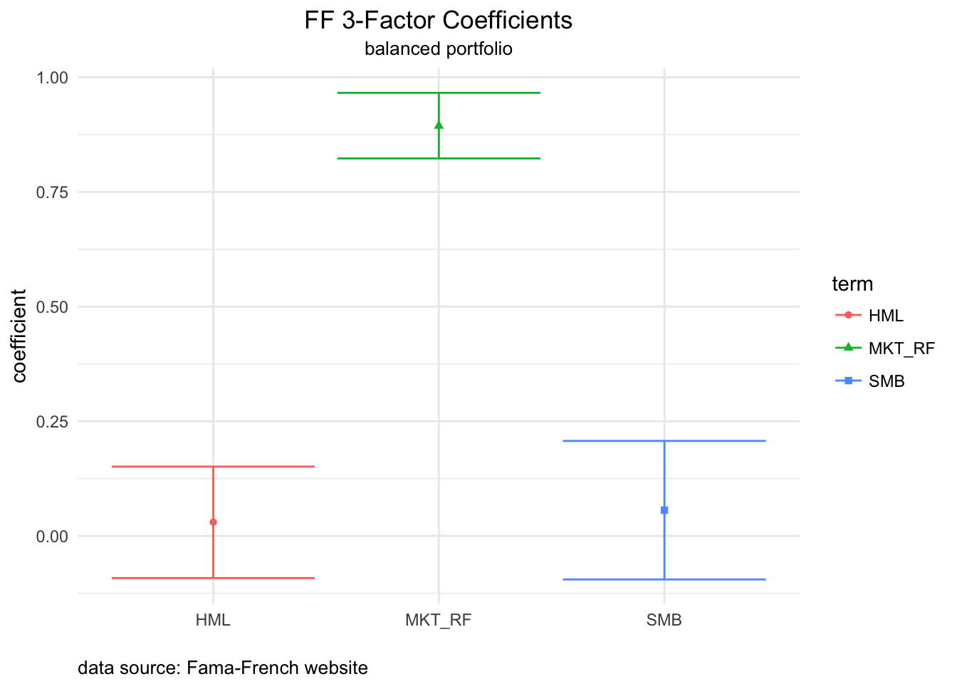
Figure 1: Fama-French factor betas
Rolling Fama-French with the tidyverse and tibbletime
# Choose a 24-month rolling window
window <- 24
# define a rolling ff model with tibbletime
rolling_lm <-
  rollify(.f = function(R_excess, MKT_RF, SMB, HML) {
  lm(R_excess ~ MKT_RF + SMB + HML)
  }, window = window, unlist = FALSE)
rolling_ff_betas <-
ff_portfolio_returns %>%
mutate(rolling_ff =
rolling_lm(R_excess,
MKT_RF,
SMB,
HML)) %>%
slice(-1:-23) %>%
select(date, rolling_ff)
head(rolling_ff_betas, 3)## # A tibble: 3 x 2
## date rolling_ff
## <date> <list>
## 1 2014-12-31 <S3: lm>
## 2 2015-01-31 <S3: lm>
## 3 2015-02-28 <S3: lm>rolling_ff_betas <-
ff_portfolio_returns %>%
mutate(rolling_ff =
rolling_lm(R_excess,
MKT_RF,
SMB,
HML)) %>%
mutate(tidied = map(rolling_ff,
tidy,
conf.int = T)) %>%
unnest(tidied) %>%
slice(-1:-23) %>%
select(date, term, estimate, conf.low, conf.high) %>%
filter(term != "(Intercept)") %>%
rename(beta = estimate, factor = term) %>%
group_by(factor)
head(rolling_ff_betas, 3)## # A tibble: 3 x 5
## # Groups: factor [3]
## date factor beta conf.low conf.high
## <date> <chr> <dbl> <dbl> <dbl>
## 1 2014-12-31 MKT_RF 0.931 0.784 1.08
## 2 2014-12-31 SMB -0.0130 -0.278 0.252
## 3 2014-12-31 HML -0.160 -0.459 0.139rolling_ff_rsquared <-
ff_portfolio_returns %>%
mutate(rolling_ff =
rolling_lm(R_excess,
MKT_RF,
SMB,
HML)) %>%
slice(-1:-23) %>%
mutate(glanced = map(rolling_ff,
glance)) %>%
unnest(glanced) %>%
select(date, r.squared, adj.r.squared, p.value)
head(rolling_ff_rsquared, 3)## # A tibble: 3 x 4
## date r.squared adj.r.squared p.value
## <date> <dbl> <dbl> <dbl>
## 1 2014-12-31 0.898 0.883 4.22e-10
## 2 2015-01-31 0.914 0.901 8.22e-11
## 3 2015-02-28 0.919 0.907 4.19e-11Visualizing Rolling Fama-French
rolling_ff_betas %>%
  ggplot(aes(x = date,
             y = beta,
             color = factor)) +
  geom_line() +
  labs(title= "24-Month Rolling FF Factor Betas") +
  theme_minimal() +
  theme(plot.title = element_text(hjust = 0.5),
axis.text.x = element_text(angle = 90)) 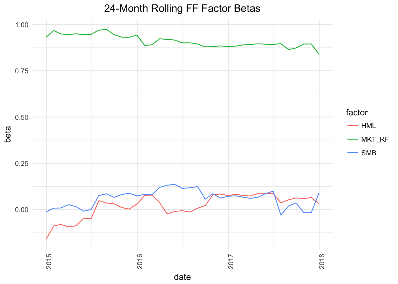
Figure 2: Rolling Factor Betas
rolling_ff_rsquared_xts <-
  rolling_ff_rsquared %>%
  tk_xts(date_var = date, silent = TRUE)
highchart(type = "stock") %>%
hc_add_series(rolling_ff_rsquared_xts$r.squared,
color = "cornflowerblue",
name = "r-squared") %>%
hc_title(text = "Rolling FF 3-Factor R-Squared") %>%
hc_add_theme(hc_theme_flat()) %>%
hc_navigator(enabled = FALSE) %>%
hc_scrollbar(enabled = FALSE) %>%
hc_exporting(enabled = TRUE)highchart(type = "stock") %>%
hc_add_series(rolling_ff_rsquared_xts$r.squared,
color = "cornflowerblue",
name = "r-squared") %>%
hc_title(text = "Rolling FF 3-Factor R-Squared") %>%
hc_yAxis( max = 2, min = 0) %>%
hc_add_theme(hc_theme_flat()) %>%
hc_navigator(enabled = FALSE) %>%
hc_scrollbar(enabled = FALSE) %>%
hc_exporting(enabled = TRUE)