Sharpe Ratio in the tidyverse

sharpe_tidyverse_byhand <- 
  portfolio_returns_dplyr_byhand %>% 
  summarise(sharpe_dplyr = mean(returns - rfr)/
              sd(returns - rfr))

sharpe_tidyverse_byhand

## # A tibble: 1 x 1
##   sharpe_dplyr
##          <dbl>
## 1        0.275

Shape Ratio in the tidyquant world

sharpe_tq <- 
  portfolio_returns_tq_rebalanced_monthly %>%
  tq_performance(Ra = returns,
                 performance_fun = SharpeRatio,
                 Rf = rfr,
                 FUN= "StdDev") %>%
  `colnames<-`("sharpe_tq")

sharpe_tq %>% 
  mutate(tidy_sharpe = sharpe_tidyverse_byhand$sharpe_dplyr,
         xts_sharpe = sharpe_xts)

## # A tibble: 1 x 3
##   sharpe_tq tidy_sharpe xts_sharpe
##       <dbl>       <dbl>      <dbl>
## 1     0.275       0.275      0.275

market_returns_xts <- 
    getSymbols("SPY", 
               src = 'yahoo', 
               from = "2012-12-31", 
               to = "2017-12-31", 
               auto.assign = TRUE, 
               warnings = FALSE) %>% 
    map(~Ad(get(.))) %>% 
    reduce(merge) %>%
    `colnames<-`("SPY") %>% 
    to.monthly(indexAt = "lastof", 
               OHLC = FALSE)

market_sharpe <- 
  market_returns_xts %>%
  tk_tbl(preserve_index = TRUE, 
         rename_index = "date") %>%
    mutate(returns = 
             (log(SPY) - log(lag(SPY)))) %>% 
    na.omit() %>% 
    summarise(ratio = 
                mean(returns - rfr)/sd(returns - rfr))

market_sharpe$ratio

## [1] 0.43475

Visualizing Sharpe Ratio

sharpe_byhand_with_return_columns <- 
  portfolio_returns_tq_rebalanced_monthly %>% 
  mutate(ratio = 
           mean(returns - rfr)/sd(returns - rfr)) %>%  
  mutate(returns_below_rfr = 
           if_else(returns < rfr, returns, as.numeric(NA))) %>%
  mutate(returns_above_rfr = 
           if_else(returns > rfr, returns, as.numeric(NA))) %>% 
  mutate_if(is.numeric, funs(round(.,4)))

sharpe_byhand_with_return_columns %>% 
  head(3)

## # A tibble: 3 x 5
##   date       returns ratio returns_below_rfr returns_above_rfr
##   <date>       <dbl> <dbl>             <dbl>             <dbl>
## 1 2013-01-31  0.0308 0.275           NA                 0.0308
## 2 2013-02-28 -0.0009 0.275           -0.0009           NA     
## 3 2013-03-31  0.0187 0.275           NA                 0.0187

sharpe_byhand_with_return_columns %>% 
  ggplot(aes(x = date)) +
  geom_point(aes(y = returns_below_rfr), 
             colour = "red") +
  geom_point(aes(y = returns_above_rfr), 
             colour = "green") + 
  geom_vline(xintercept = 
               as.numeric(as.Date("2016-11-30")), 
             color = "blue") +
  geom_hline(yintercept = rfr, 
             color = "purple", 
             linetype = "dotted") +
  annotate(geom = "text", 
           x = as.Date("2016-11-30"), 
           y = -.04, 
           label = "Election", 
           fontface = "plain", 
           angle = 90, 
           alpha = .5, 
           vjust =  1.5) +
  ylab("percent monthly returns") +
  scale_y_continuous(breaks = pretty_breaks(n = 10)) +
  scale_x_date(breaks = pretty_breaks( n = 8))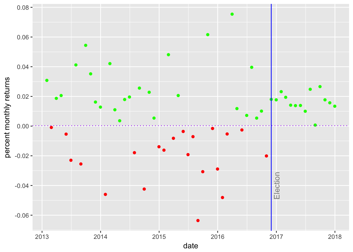

Figure 1: Scatter Returns Around Risk Free Rate

sharpe_byhand_with_return_columns %>% 
  ggplot(aes(x = returns)) +
  geom_histogram(alpha = 0.45, 
                 binwidth = .01, 
                 fill = "cornflowerblue") +
  geom_vline(xintercept = rfr, 
             color = "green") +
  annotate(geom = "text", 
           x = rfr,
           y = 13, 
           label = "rfr", 
           fontface = "plain", 
           angle = 90, 
           alpha = .5, 
           vjust =  1)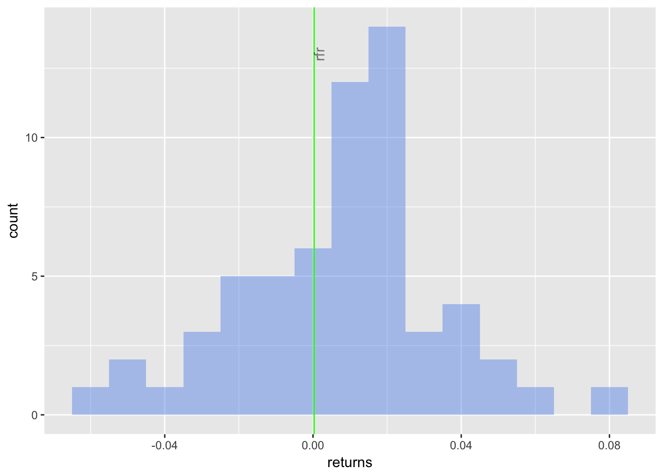

Figure 2: Returns Histogram with Risk-Free Rate ggplot

asset_returns_long %>% 
  group_by(asset) %>% 
  summarise(stand_dev = sd(returns),
            sharpe = mean(returns - rfr)/
              sd(returns - rfr))%>% 
  add_row(asset = "Portfolio",
    stand_dev = 
      portfolio_sd_xts_builtin[1],
    sharpe = 
      sharpe_tq$sharpe_tq) %>% 
  ggplot(aes(x = stand_dev, 
             y = sharpe, 
             color = asset)) +
  geom_point(size = 2) +
  geom_text(
   aes(x = 
    sd(portfolio_returns_tq_rebalanced_monthly$returns), 
     y = 
    sharpe_tq$sharpe_tq + .02, 
         label = "Portfolio")) +
  ylab("Sharpe") +
  xlab("standard deviation") +
  ggtitle("Sharpe Ratio versus Standard Deviation") +
  # The next line centers the title
  theme_update(plot.title = element_text(hjust = 0.5))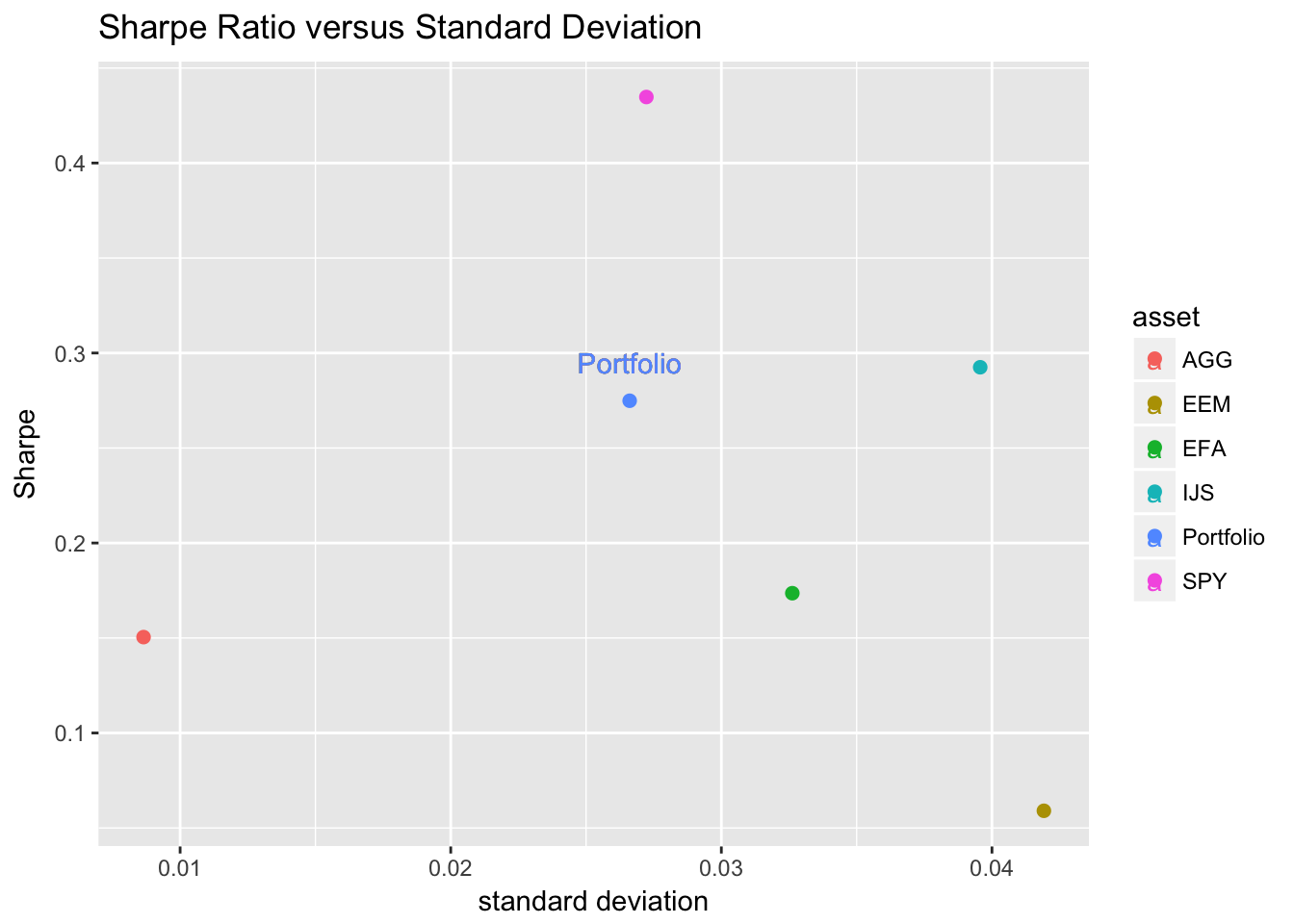

Figure 3: Sharpe v. Standard Deviation

Rolling Sharpe Ratio in the xts world

window <- 24

rolling_sharpe_xts <- 
  rollapply(portfolio_returns_xts_rebalanced_monthly, 
            window, 
            function(x) 
            SharpeRatio(x, 
                        Rf = rfr, 
                        FUN = "StdDev")) %>% 
  na.omit() %>% 
  `colnames<-`("xts")

Rolling Sharpe Ratio with the tidyverse and tibbletime

# Creat rolling function.
sharpe_roll_24 <- 
  rollify(function(returns) {
    ratio = mean(returns - rfr)/sd(returns - rfr)
    }, 
window = window)

rolling_sharpe_tidy_tibbletime <- 
  portfolio_returns_dplyr_byhand %>%
  as_tbl_time(index = date) %>% 
  mutate(tbltime_sharpe = sharpe_roll_24(returns)) %>% 
  na.omit() %>%
  select(-returns)

Rolling Sharpe Ratio with tidyquant

sharpe_tq_roll <- function(df){
  SharpeRatio(df, 
              Rf = rfr, 
              FUN = "StdDev")
}

rolling_sharpe_tq <-
portfolio_returns_tq_rebalanced_monthly %>% 
tq_mutate(
        select     = returns,
        mutate_fun = rollapply, 
        width      = window,
        align      = "right",
        FUN        = sharpe_tq_roll,
        col_rename = "tq_sharpe"
    ) %>% 
  na.omit()

rolling_sharpe_tidy_tibbletime %>% 
 mutate(xts_sharpe = coredata(rolling_sharpe_xts),
        tq_sharpe = rolling_sharpe_tq$tq_sharpe ) %>% 
  head(3)

## # A time tibble: 3 x 4
## # Index: date
##   date       tbltime_sharpe xts_sharpe tq_sharpe
##   <date>              <dbl>      <dbl>     <dbl>
## 1 2014-12-31          0.312      0.312     0.312
## 2 2015-01-31          0.237      0.237     0.237
## 3 2015-02-28          0.300      0.300     0.300

Visualizing the Rolling Sharpe Ratio

highchart(type = "stock") %>%
  hc_title(text = "Rolling  24-Month Sharpe") %>%
  hc_add_series(rolling_sharpe_xts, 
                name = "sharpe", 
                color = "blue") %>%
  hc_navigator(enabled = FALSE) %>% 
  hc_scrollbar(enabled = FALSE) %>% 
  hc_add_theme(hc_theme_flat()) %>%
  hc_exporting(enabled = TRUE)

rolling_sharpe_xts %>% 
  tk_tbl(preserve_index = TRUE, 
         rename_index = "date") %>%
  rename(rolling_sharpe = xts) %>% 
  ggplot(aes(x = date, 
             y = rolling_sharpe)) +
  geom_line(color = "cornflowerblue") +
  ggtitle("Rolling 24-Month Sharpe Ratio") +
  labs(y = "rolling sharpe ratio") +
  scale_x_date(breaks = pretty_breaks(n = 8)) +
   theme(plot.title = element_text(hjust = 0.5))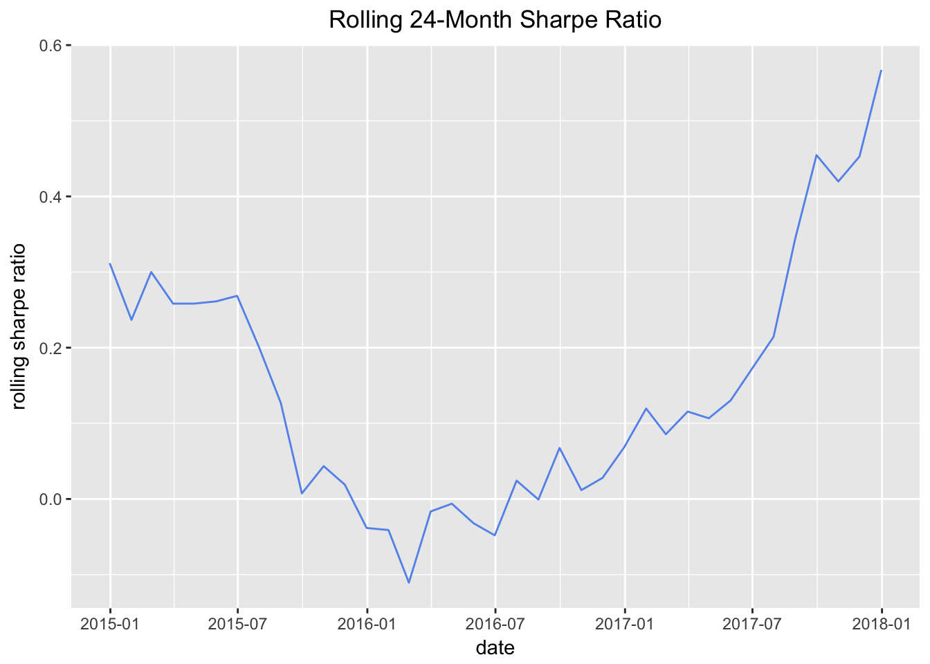

Figure 4: Rolling Sharpe ggplot